In this post, I will explain how to embed a QlikView dashboard into an OBIEE dashboard page.
This can be useful if you have a scenario where OBI is your primary platform, but there are also dashboards built in QlikView or some other BI Platform, and you want to direct the users to one place for all dashboards instead of having to explain to them to “go here for this, and there for that”.
So, I am assuming you already have a QlikView dashboard built that you would like to embed into OBIEE.
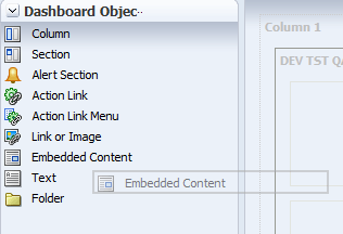
Create or edit your OBIEE dashboard page. While on the page in edit mode, drop in/drag in an “Embedded Content” object.
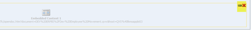
With the Embedded Content Object on the dashboard page in Edit mode, edit the “Embedded Content” Object.
In the Embedded Content Properties dialog …
– Enter the URL to your QlikView dashboard
– Check the box for “This URL Embeds an Application”
– and enter the Width and Height you desire for the embedded area.
– Optionally, check the box for “Hide Scroll Bars”. Make sure not to check this box if your dashboard is vertically longer than a typical monitor.
Click OK, and then Save your dashboard page.
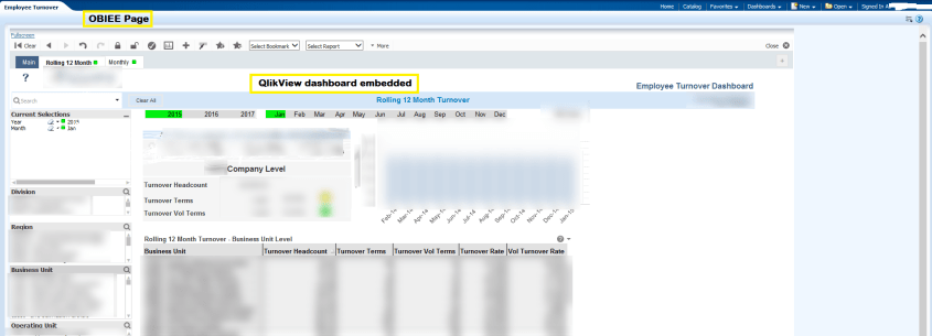
When you now open your dashboard in OBIEE, you will see your QlikView dashboard embedded within the page.
Thanks for reading! I hope you found this article useful.
In QlikView, there is the CONCATENATE statement, the CONCAT() function, and the string concatenation operator (the ampersand – &). These are all very different and in this post I will explain each of them.
CONCATENATE statement
The CONCATENATE statement is used in conjunction with the LOAD statement. It appends the rows of one table to another. It is similar to a UNION ALL statement in SQL.
Let’s take a look at a couple examples using the following tables:
Employee_Location
Employee_ID
Employee_Name
Employee_Location
1
John
NY
2
Mary
NJ
Employee_Office
Employee_ID
Employee_Name
Employee_State
3
Jane
FL
4
Evan
NY
Employee_Position
Employee_ID
Employee_Name
Employee_Position
5
Paul
Cashier
6
Sonia
Salesperson
If we concatenated the Employee_Location and Employee_Office tables using the following load script …
[Employee_Location]:
 LOAD
 [Employee_ID]       as [%Employee ID],
 [Employee_Name]     as [Employee Name],
 [Employee_Location] as [Employee Location]
 FROM [… data source details for Employee_Location …]

CONCATENATE (Employee_Location)
 LOAD
 [Employee_ID]        as [%Employee ID],
 [Employee_Name]      as [Employee Name],
 [Employee_State]     as [Employee Location]  --aliased column
 FROM [… data source details for Employee_Office …]
We would get this result …
Employee_Location
Employee ID
Employee Name
Employee Location
1
John
NY
2
Mary
NJ
3
Jane
FL
4
Evan
NY
Now, if we concatenated the Employee_Location and Employee_Position tables using the following script…
[Employee_Information]:
 LOAD
 [Employee_ID]       as [%Employee ID],
 [Employee_Name]     as [Employee Name],
 [Employee_Location] as [Employee Location]
 FROM [… data source details for Employee_Location …]

CONCATENATE (Employee_Information)
 LOAD
 [Employee_ID]        as [%Employee ID],
 [Employee_Name]      as [Employee Name],
 [Employee_Position]  as [Employee Position]
 FROM [… data source details for Employee_Position …]
We would get this result …
Employee_Information
Employee ID
Employee Name
Employee Location
Employee Position
1
John
NY
2
Mary
NJ
5
Paul
Cashier
6
Sonia
Salesperson
Notice that the concatenation works even if the tables do not have the same number of columns. This provide more flexibility than the UNION or UNION ALL statements in SQL where you need to add a dummy column to the select list of your first table before performing the union.
Concat() function
The concat() function concatenates all the values of a column into a single delimited string. The column and the delimiter are specified as parameters in the function. You also have the option of producing the result string with only distinct values.
For example, if you have the following table …
Product_ID
Product_Description
Product_Category
1212
Pen
Office Supplies
3214
Paper
Paper
1345
Sharpener
Office Supplies
1177
Eraser
Office Supplies
2780
Calculator
Electronics
2901
Computer
Electronics
This statement: CONCAT(Product_Category, ‘,’)
Produces: Electronics, Electronics, Office Supplies, Office Supplies, Office Supplies, Paper Notice there is a space after the comma in the delimiter, and therefore, there is a space after the comma in the output
This statement: CONCAT(Product_Category, ‘|’)
Produces: Electronics|Electronics|Office Supplies|Office Supplies|Office Supplies|Paper Notice there is no space in the delimiter, and therefore, no space between the values in the output
This statement: CONCAT(DISTINCT Product_Category, ‘ | ’)
Produces: Electronics | Office Supplies | Paper Notice spaces in the delimiter, and distinct output.
Concatenation operator ( & )
When you need to concatenate 2 strings together, you use the concatenation operator – the ampersand (&). For example, if you have address values in separate columns as in the table below …
Street
City
State
Zip
123 Main St
Orlando
FL
32801
… you can output the address as one concatenated string by using the concatenation operator as shown in the script below …
[Street] & ‘, ‘ & [City] & ‘, ‘ & [State] & ‘ ‘ & [Zip]

[Notice a comma and a space is concatenated between Street, City and State;
and only a space is concatenate between State and Zip]
… and that would produce the following result … 123 Main St, Orlando, FL 32801
With the expansion of Self-Service BI, BI Teams need to be more vigilant about protecting sensitive data.
This is a summary of options available for protecting data in Oracle databases.
The information in this post was found here and summarized for a quick read: https://docs.oracle.com/database/121/ASOAG/toc.htm
The 3 features available are (1) Transparent Data Encryption, (2) Data Redaction, and (3) Data Masking and Subsetting Pack.
Here is a quick summary.
(1) Transparent Data Encryption (TDE)
Encrypt data so only authorized people can see it
Use it to protect sensitive data that maybe in an unprotected environment, such backup data sent to a storage facility
You can encrypt an individual column or an entire tablespace
Applications using encrypted data can function just the same
(2) Data Redaction
Enable the redaction (masking) of column data in tables
Redaction can be full, partial, based on regular expressions, or random
Full redaction: replaces strings with a single blank space ‘ ‘; numbers with zero (0); dates with 01-JAN-01
Partial redaction: replaces a portion of the column data; for example SSN: ***-**-1234
Regular expressions: can be used to perform partial or full redactions
Random: generates random values for display when accessed
The redaction takes place at runtime; not in the permanent data stored
(3) Oracle Enterprise Manager Data Masking and Subsetting Pack
enables you to create a “safe” development or test copy of the production database
Let’s look into some more details …
(1) Transparent Data Encryption (TDE)
TDE uses a two-tiered key-based architecture
TDE column encryption uses the two-tiered key-based architecture to transparently encrypt and decrypt sensitive table columns. The TDE master encryption key is stored in an external security module, which can be an Oracle software keystore or hardware keystore. This TDE master encryption key encrypts and decrypts the TDE table key, which in turn encrypts and decrypts data in the table column.
A Key Management Framework is used for TDE to store and manage keys and credentials.
Includes the keystore to store the TDE master encryption keys and the management framework to manage keystore and key operations
The Oracle keystore stores a history of retired TDE master encryption keys, which enables you to change them and still be able to decrypt data that was encrypted under an earlier TDE master encryption key.
Types of Keystores
Software keystores
Hardware, or HSM-based, keystores
Types of Software Keystores:
auto-login software keystores that are local to the computer on which they are created.
cannot be opened on any computer other than the one on which they are created.
typically used for scenarios where additional security is required while supporting an unattended operation
Password-based software keystores
protected by using a password that you create. You must open this type of keystore before the keys can be retrieved or used.
Auto-login software keystores
protected by a system-generated password, and do not need to be explicitly opened; automatically opened when accessed.
can be used across different systems; ideal for unattended scenarios.
Local auto-login software keystores
Steps for configuring a Software Keystore
Step 1: Set the Software Keystore Location in the sqlnet.ora File
Step 2: Create the Software Keystore
Step 3: Open the Software Keystore
Step 4: Set the Software TDE Master Encryption Key
Step 5: Encrypt Your Data
Oracle Database checks the sqlnet.ora file for the directory location of the keystore, whether it is a software keystore or a hardware module security (HSM) keystore.
You cannot change an existing tablespace to make it encrypted
You can create or modify columns to be encrypted
(2) Data Redaction
Define data redaction policies to specify what data needs to be redacted
Use policy expressions to set whether a user sees the redacted data or the full data
Policy Procedures
DBMS_REDACT.ADD_POLICY
DBMS_REDACT.ALTER_POLICY
DBMS_REDACT.ENABLE_POLICY
DBMS_REDACT.DISABLE_POLICY
DBMS_REDACT.DROP_POLICY
Sample scrip
BEGIN
DBMS_REDACT.ADD_POLICY(
object_schema => ‘hr’,
object_name => ’employees’,
column_name => ‘commission_pct’,
policy_name => ‘redact_com_pct’,
function_type => DBMS_REDACT.PARTIAL, –partial; use DBMS_REDACT.FULL for full
function_parameters => DBMS_REDACT.REDACT_US_SSN_F5, — many standard params, but it can also be custom
expression => ‘SYS_CONTEXT(”SYS_SESSION_ROLES”,”MGR”) = ”FALSE”’); –allows MGR role to see data
policy_description => ‘Partially redacts 1st 5 digits in SS numbers’,
column_description => ‘ssn contains Social Security numbers’);
END;
/
Use DBMS_REDACT.ALTER_POLICY and action => DBMS_REDACT.ADD_COLUMN to redact multiple columns
Redaction takes place on select lists and not on where clauses
Be aware of the scenarios when using redacted tables to build other tables or views
(3) Oracle Enterprise Manager Data Masking and Subsetting Pack (DMSP)
DMSP enables you to create a development or test copy of the production database, by taking the data in the production database, masking this data in bulk, and/or creating a subset of the data, and then putting the resulting masked data and/or subset of data in the development or test copy.
You can still apply Data Redaction policies to the non-production database, in order to redact columns
Used to mask data sets when you want to move the data to development and test environments.
Data Redaction is mainly designed for redacting at runtime for production applications
——–
I hope you found this helpful to get you started on taking the steps to protect your data internally and externally.
You can visit the link I provided above to find more details.
When your Oracle Business Intelligence Applications (OBIA) DAC Execution Plan fails with a message that looks like this …
“Retrieving execution plan informationMESSAGE:::com.siebel.analytics.etl.execution.exceptions.EmptyExecutionPlanException: No active subject areas for execution plan were found EXCEPTION CLASS::: com.siebel.analytics.etl.execution.ExecutionPlanInitializationException
It is likely that you have a missing Subject Area in your Execution Plan in DAC. You need to attach the Subject Area to the Execution Plan and rebuild the Plan.
After doing this your job should run successfully.
In this post, I will show the steps for using the OBIEE “Repository Documentation” utility to generate repository (RPD) lineage information. I will also provide a couple example of how this documentation (output file) can be used.
To access and run the Repository Documentation utility, from the BI Admin Tool menu, select Tools -> Utilities.
From the Utilities dialog, select “Repository Documentation”, and click “Execute…”
In the “Save As” dialog, select the destination and enter the name you would like for the output file.
When it finishes, it will generate the output csv file. Note – this will likely be a large file. It will contain all your repository objects.
You can use this file to quickly track lineage from physical sources to the logical columns to the presentation columns and identify all the logic and variables in between.
You can also use it to identify where and how much a specified table, column, variable, etc. is used which will help you to identify dependencies and know the effect of making changes or deleting elements.
Development, Data Governance, and Quality Assurance teams may find this information useful in this format.
This post covers the basics of navigation and selection for getting data into your Qlik Sense application. More information about each option will be detailed in upcoming posts.
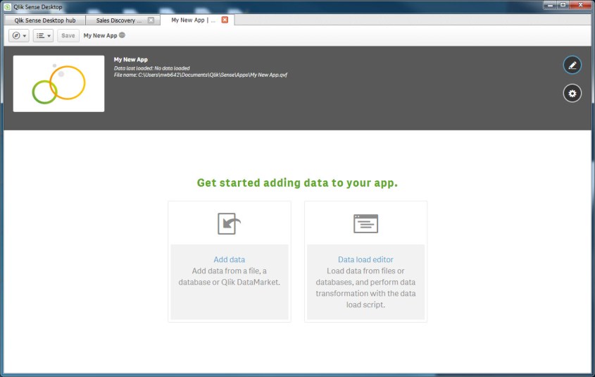
When you are working with a new app to which data has not yet been loaded, with the app open you can use the “Add data” or “Data load editor” icons shown below the app title area to initiate a data load.
Use the “Add data” icon to add data from a file, database, or Qlik DataMarket using the Quick Data Load (QDL) wizard.
Use the “Data load editor” (DLE) to load data from files or databases, and perform data transformation with data load scripts.
If your app already has data, the area below the app title area will contain existing Sheets, Bookmarks, and Stories. But you will still be able to access the QDL and the DLE.
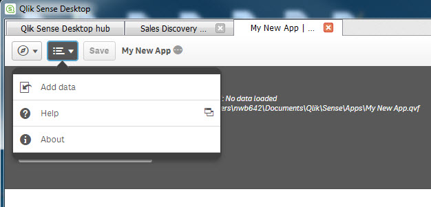
For the QDL wizard, you can access it from the Global Menu, and select the “Add data” menu item.
For the DLE, you can access it from the Navigation menu, and select the “Data load editor” menu item.
More details about what comes next will be in upcoming posts.
When you start Qlik Sense, it will open to the “hub” page. And you may also see a “Welcome…” dialog window.
From the “Welcome …” window, you may click the “Create a new App” button to start the process of creating a new app, or click the “x” in the top-right to close the window.
Optionally, you may uncheck the “Show this dialog at startup” checkbox before closing it, if you do not want to show this window on each startup of Qlik Sense. If this was unchecked previously, then this Welcome dialog would not have appeared.
Once you have closed the Welcome dialog, you will then be in the main hub interface. Let’s take a look at it.
At the top left, you will see the Global Menu. From this menu you can access Help and About, and also access the Dev Hub. The Global Menu expanded is shown below.
Below the Global Menu is the Apps area. Here you will see the applications that have been created and saved.
At the bottom of the page, you will see a “Getting started…” button. Clicking here will bring you to a Qlik Sense support page containing information and resources to help you get started with Qlik Sense.
To the right in the main area of the window, there is a “Create new app” button which you will use when you need to create a new app.
Then, there is an icon for sorting the apps alphabetically – ascending or descending. Then, another pair of icons for organizing the display of the apps – either in grid format or in list format.
Above that (top-right), you will find the icon for Qlik Cloud, and another icon for Search.
Data Science is very complementary to Business Intelligence, in that they are both used to gain insights from data. While Business Intelligence, generally speaking, is more about answering known questions, Data Science is more about discovery and providing information for previously unknown questions.
This is a continuation of a series of Data Science Fundamentals posts that I will be doing over the next few weeks. In this post, I will be covering Regression and will include an example to make it more meaningful. Previous posts covered Classification and Clustering. Upcoming posts over the next few days will cover Matching, and other data science fundamental concepts.
Regression analysis is a predictive modeling technique which investigates the relationship between a dependent or target variable and one or more independent or predictor variables. It can be used to predict the value of a variable and the class the variable belongs to and identifies the strength of the relationships and the strength of impact between the variables. There are many variations of regression with linear and logistic regression being the most commons methods used. The various regression methods will be explored at a later point in time.
An example of how Regression can be used is, you may identify products similar to a given product, that is, products that are in the same class or category as your subject product. Then review the historical performance of those similar products under certain promotions, and use that to estimate/predict how well the subject product will perform under similar promotions.
Another example is, you may use the classification of a customer or prospect to estimate/predict how much that customer/prospect is likely to spend on your products and services each year.
Classification determines the group/class of an entity, whereas Regression determines where on the spectrum (expressed as a numerical value) of that class the entity falls. An example using a hotel customer – Classification: Elite Customer; Regression: 200 nights per year (on a scale of 100-366 nights per year) or top 10% of customers.
Like Business Intelligence, the essential purpose of Data Science is to gain knowledge and insights from data. This knowledge can then be used for a variety of purposes – such as, driving more sales, retaining more employees, reducing marketing costs, and saving lives.
This is a continuation of a series of Data Science Fundamentals posts that I will be doing over the next few weeks. In this post, I will be covering Clustering and will include an example to make it more meaningful. A previous post covered Classification. Upcoming posts over the next few days will cover Regression, Matching, and other data science fundamental concepts.
Clustering is similar to Classification, in that, they are both used to categorize and segment data. But Clustering is different from Classification, in that, clustering segments the data into groups (clusters) not previously defined or even known in some cases. Clustering explores the data and finds natural groupings/clusters/classes without any targets (previously defined classes). This is called “unsupervised” segmentation. It clusters the data entities based on some similarity that makes them more like each other than entities in other clusters. Therefore, this is a great first step if information about the data set is unknown.
Clustering: 3 clusters formed (with an outlier)
The Clustering process may yield clusters/groups than can be later used for Classification. Using the defined classes as targets is called “supervised” segmentation. In the diagram to the right, there are 3 clusters that have been formed (red pluses, blue circles, green diamonds).
After a Clustering process is completed, there may be some data entities that are clustered by themselves. In other words, they do not fall into any of the other clusters containing multiple entities. These are classified as outliers. An example of this can be seen in the diagram where there is an outlier in the top-left corner (purple square). Analysis on these outliers can sometimes yield additional insight.
Software such as R and Python provides functions for performing cluster analysis/segmentation on datasets. Future posts will cover these topics along with more details on Clustering.
Over the next 3 months, I will be focusing on Data Science and my next few posts will cover some fundamental topics of Data Science.
The essential purpose of Data Science, like Business Intelligence, is to gain knowledge and insights from data. This knowledge can then be used for a variety of purposes – such as, driving more sales, retaining more employees, reducing marketing costs, and saving lives.
In this post, I will be covering Classification and will include examples to make it more meaningful. Upcoming posts over the next few days will cover Clustering, Regression, Matching, and other data science fundamental concepts.
Classification is the process of using characteristics, features, and attributes of a data entity (such as a person, company, or thing) to determine what class (group or category) it belongs to and assigning it to that class. As an example, demographic data is usually a classification – marital status (married, single, divorced), income bracket (wealthy, middle-class, poor), homeowner status (homeowner or renter), age bracket (old, middle-aged, young), etc.
Shapes are classified by characteristics such as number of sides, length of sides, etc.
When a large amount of data needs to be analyzed, Classification needs to be an automated process. If the classes are not know ahead of time, a process called Clustering can be used on existing data to discover groups that can in some way be used to form the classes.(Clustering will be covered in an upcoming post)
Class Probability Estimation (Scoring) is the process of producing a score that represents the probability of the data entity being in a particular class. As an example, Income Bracket – top 5%.
A few Use Cases and examples of Classification and Class Probably Estimation/Scoring are:
(1) Financial: credit risk – High-Risk, Medium-Risk, Low-Risk, Safe.
A person’s past credit history (or lack of one) will determine their credit score. And their credit score will determine what class of credit risk they fall into, and therefore, will determine if they get the loan, and how favorable the terms of the loan would be.
As an example of Class Probability Estimation (Scoring) for this use case, a person may fall in the Low-Risk class, but their credit score (sometime called FICO score) shows that they are in the low-end of the Low-Risk class making them bordering on Medium-Risk.
(2) Marketing: Marketing offer/promotion interest – Highly likely, Likely, Unlikely
Based on past promotions and those who responded to it, classification can be used to determine the likelihood of a person being interested in a specific marketing offer/promotion. This is known as targeted marketing where specific promotions are sent only to those who will likely be interested, and therefore, different classes/groups may receive different marketing messages from the same company.
As an example of Class Probability Estimation (Scoring) for this use case, a customer or prospect could be scored as 70% Unlikely, or 90% Highly Likely.
(3) Customer Base: Top-customer, Seasonal Customer, Loyal customer, High-Chance of Losing customer, …
A company may use some set of criteria to classify customers into various categories. These categories can be used for various customer-focused efforts, such as marketing, special offers, rewards, and more.
(4) Fraud detection & security: Transaction or Activity occurrence – Highly Unusual, Unusual, Normal
Based on past activity and all other activities as a whole, a person’s activity/transaction can be classified as unusual or normal, and the appropriate actions taken to protect their accounts.
(5) Healthcare:
Data from past health analysis and treatments can be used to classify the level of a patient’s illness, and classify their treatment class. This will then drive the recommended treatment.
(6) Human behavior/Workforce:
Today’s workforce consists of multiple generations (Baby Boomers, GenX, GenY/Millennials, etc) of workers. Generational classification of people based on the period in which they were born is used for marketing purposes, but is also used to help educate a diverse workforce on understanding their team members of different generations and how to work with them.
There are of course many more types of classification and use cases. Feel free to share your use cases.
Information and resources for the data professionals' community


 From the “Welcome …” window, you may click the “Create a new App” button to start the process of creating a new app, or click the “x” in the top-right to close the window.

 It can be used to predict the value of a variable and the class the variable belongs to and identifies the strength of the relationships and the strength of impact between the variables. There are many variations of regression with linear and logistic regression being the most commons methods used. The various regression methods will be explored at a later point in time.

