Category: Analytics

Create and Update Reusable Assets, including Power BI template (.pbit) files, Power BI data source (.pbids) files, and shared semantic models in Microsoft Fabric

This post is a part of the DP-600: Implementing Analytics Solutions Using Microsoft Fabric Exam Prep Hub; and this topic falls under these sections: 
Maintain a data analytics solution
--> Maintain the analytics development lifecycle
--> Create and update reusable assets, including Power BI template (.pbit)
files, Power BI data source (.pbids) files, and shared semantic models

Reusable assets are a key lifecycle concept in Microsoft Fabric and Power BI. They enable consistency, scalability, and efficiency by allowing teams to standardize how data is connected, modeled, and visualized across multiple solutions.

For the DP-600 exam, you should understand what reusable assets are, how to create and manage them, and when each type is appropriate.

What Are Reusable Assets?

Reusable assets are analytics artifacts designed to be:

  • Used by multiple users or teams
  • Reapplied across projects
  • Centrally governed and maintained

Common reusable assets include:

  • Power BI template (.pbit) files
  • Power BI data source (.pbids) files
  • Shared semantic models

Power BI Template Files (.pbit)

What Is a PBIT File?

A .pbit file is a Power BI template that contains:

  • Report layout and visuals
  • Data model structure (tables, relationships, measures)
  • Parameters and queries (without data)

It does not include actual data.

When to Use PBIT Files

PBIT files are ideal when:

  • Standardizing report design and metrics
  • Distributing reusable report frameworks
  • Supporting self-service analytics at scale
  • Onboarding new analysts

Creating and Updating PBIT Files

  • Create a report in Power BI Desktop
  • Remove data (if present)
  • Save as Power BI Template (.pbit)
  • Store in source control or shared repository
  • Update centrally and redistribute as needed

Power BI Data Source Files (.pbids)

What Is a PBIDS File?

A .pbids file is a JSON-based file that defines:

  • Data source connection details
  • Server, database, or endpoint information
  • Authentication type (but not credentials)

Opening a PBIDS file launches Power BI Desktop and guides users through connecting to the correct data source.

When to Use PBIDS Files

PBIDS files are useful for:

  • Standardizing data connections
  • Reducing configuration errors
  • Guiding business users to approved sources
  • Supporting governed self-service analytics

Managing PBIDS Files

  • Create manually or export from Power BI Desktop
  • Store centrally (e.g., Git, SharePoint)
  • Update when connection details change
  • Pair with shared semantic models where possible

Shared Semantic Models

What Are Shared Semantic Models?

Shared semantic models are centrally managed datasets that:

  • Define business logic, measures, and relationships
  • Serve as a single source of truth
  • Are reused across multiple reports

They are one of the most important reusable assets in Fabric.

Benefits of Shared Semantic Models

  • Consistent metrics across reports
  • Reduced duplication
  • Centralized governance
  • Better performance and manageability

Managing Shared Semantic Models

Shared semantic models are:

  • Developed by analytics engineers
  • Published to Fabric workspaces
  • Shared using Build permission
  • Governed with:
    • RLS and OLS
    • Sensitivity labels
    • Endorsements (Promoted/Certified)

How These Assets Work Together

A common pattern:

  • PBIDS → Standardizes connection
  • Shared semantic model → Defines logic
  • PBIT → Standardizes report layout

This layered approach is frequently tested in exam scenarios.

Reusable Assets and the Development Lifecycle

Reusable assets support:

  • Faster development
  • Consistent deployments
  • Easier maintenance
  • Scalable self-service analytics

They align naturally with:

  • PBIP projects
  • Git version control
  • Development pipelines
  • XMLA-based automation

Common Exam Scenarios

You may be asked:

  • How to distribute a standardized report template → PBIT
  • How to ensure users connect to the correct data source → PBIDS
  • How to enforce consistent business logic → Shared semantic model
  • How to reduce duplicate datasets → Shared model + Build permission

Example:

Multiple teams need to create reports using the same metrics and layout.
Correct concepts: Shared semantic model and PBIT.

Best Practices to Remember

  • Centralize ownership of shared semantic models
  • Certify trusted reusable assets
  • Store templates and PBIDS files in source control
  • Avoid duplicating business logic in individual reports
  • Pair reusable assets with governance features

Key Exam Takeaways

  • Reusable assets improve consistency and scalability
  • PBIT files standardize report design
  • PBIDS files standardize data connections
  • Shared semantic models centralize business logic
  • All are core lifecycle tools in Fabric

Exam Tips

  • If a question focuses on standardization, reuse, or self-service at scale, think PBIT, PBIDS, and shared semantic models—and choose the one that matches the problem being solved.
  • Expect scenarios that test:
    • When to use PBIT vs PBIDS vs shared semantic models
    • Governance and consistency
    • Enterprise BI scalability
  • Quick memory aid:
    • PBIT = Layout + Model (no data)
    • PBIDS = Connection only
    • Shared model = Logic once, reports many

Practice Questions

Question 1 (Single choice)

What is the PRIMARY purpose of a Power BI template (.pbit) file?

A. Store report data for reuse
B. Share report layout and model structure without data
C. Store credentials securely
D. Enable real-time data refresh

Correct Answer: B

Explanation:
A .pbit file contains:

  • Report layout
  • Semantic model (tables, relationships, measures)
  • No data

It’s used to standardize report creation.


Question 2 (Multi-select)

Which components are included in a Power BI template (.pbit)? (Select all that apply.)

A. Report visuals
B. Data model schema
C. Data source credentials
D. DAX measures

Correct Answers: A, B, D

Explanation:

  • Templates include visuals, schema, relationships, and measures.
  • ❌ Credentials and data are never included.

Question 3 (Scenario-based)

Your organization wants users to quickly connect to approved data sources while preventing incorrect connection strings. Which reusable asset is BEST?

A. PBIX file
B. PBIT file
C. PBIDS file
D. Shared semantic model

Correct Answer: C

Explanation:
PBIDS files:

  • Predefine connection details
  • Guide users to approved data sources
  • Improve governance and consistency

Question 4 (Single choice)

Which statement about Power BI data source (.pbids) files is TRUE?

A. They contain report visuals
B. They contain DAX measures
C. They define connection metadata only
D. They store dataset refresh schedules

Correct Answer: C

Explanation:
PBIDS files only store:

  • Data source type
  • Server/database info
    They do NOT include visuals, data, or logic.

Question 5 (Scenario-based)

You want multiple reports to use the same curated dataset to ensure consistent KPIs. What should you implement?

A. Multiple PBIX files
B. Power BI templates
C. Shared semantic model
D. PBIDS files

Correct Answer: C

Explanation:
A shared semantic model allows:

  • Centralized logic
  • Single source of truth
  • Multiple reports connected via Live/Direct Lake

Question 6 (Multi-select)

Which benefits are provided by shared semantic models? (Select all that apply.)

A. Consistent calculations across reports
B. Reduced duplication of datasets
C. Independent refresh schedules per report
D. Centralized security management

Correct Answers: A, B, D

Explanation:

  • Shared models enforce consistency and reduce maintenance.
  • ❌ Refresh is managed at the model level, not per report.

Question 7 (Scenario-based)

You update a shared semantic model’s calculation logic. What is the impact?

A. Only new reports see the change
B. All connected reports reflect the change
C. Reports must be republished
D. Only the workspace owner sees updates

Correct Answer: B

Explanation:
All reports connected to a shared semantic model automatically reflect changes.


Question 8 (Single choice)

Which reusable asset BEST supports report creation without requiring Power BI Desktop modeling skills?

A. PBIX file
B. PBIT file
C. PBIDS file
D. Shared semantic model

Correct Answer: D

Explanation:
Users can build reports directly on shared semantic models using existing fields and measures.


Question 9 (Scenario-based)

You want to standardize report branding, page layout, and slicers across teams. What should you distribute?

A. PBIDS file
B. Shared semantic model
C. PBIT file
D. XMLA script

Correct Answer: C

Explanation:
PBIT files are ideal for:

  • Visual consistency
  • Reusable layouts
  • Standard filters and slicers

Question 10 (Multi-select)

Which are BEST practices when managing reusable Power BI assets? (Select all that apply.)

A. Store PBIT and PBIDS files in version control
B. Update shared semantic models directly in production without testing
C. Document reusable asset usage
D. Combine shared semantic models with deployment pipelines

Correct Answers: A, C, D

Explanation:
Best practices emphasize:

  • Governance
  • Controlled updates
  • Documentation

❌ Direct production edits increase risk.


COUNT vs. COUNTA in Power BI DAX: When and How to Use Each

When building measures in Power BI using DAX, two commonly used aggregation functions are COUNT and COUNTA. While they sound similar, they serve different purposes and choosing the right one can prevent inaccurate results in your reports.

COUNT: Counting Numeric Values Only

The COUNT function counts the number of non-blank numeric values in a column.

DAX syntax:
COUNT ( Table[Column] )

Key characteristics of COUNT”:

  • Works only on numeric columns
  • Ignores blanks
  • Ignores text values entirely

When to use COUNT:

  • You want to count numeric entries such as:
    • Number of transactions
    • Number of invoices
    • Number of scores, quantities, or measurements
  • The column is guaranteed to contain numeric data

Example:
If Sales[OrderAmount] contains numbers and blanks, COUNT(Sales[OrderAmount]) returns the number of rows with a valid numeric amount.

COUNTA: Counting Any Non-Blank Values

The COUNTA function counts the number of non-blank values of any data type, including text, numbers, dates, and Boolean values.

DAX syntax:
COUNTA ( Table[Column] )

Key characteristics of “COUNTA”:

  • Works on any column type
  • Counts text, numbers, dates, and TRUE/FALSE
  • Ignores blanks only

When to use COUNTA:

  • You want to count:
    • Rows where a column has any value
    • Text-based identifiers (e.g., Order IDs, Customer Names)
    • Dates or status fields
  • You are effectively counting populated rows

Example:
If Customers[CustomerName] is a text column, COUNTA(Customers[CustomerName]) returns the number of customers with a non-blank name.

COUNT vs. COUNTA: Quick Comparison

FunctionCountsIgnoresTypical Use Case
COUNTNumeric values onlyBlanks and textCounting numeric facts
COUNTAAny non-blank valueBlanks onlyCounting populated rows

Common Pitfall to Avoid

Using COUNTA on a numeric column can produce misleading results if the column contains zeros or unexpected values. Remember:

  • Zero (0) is counted by both COUNT and COUNTA
  • Blank is counted by neither

If you are specifically interested in numeric measurements, COUNT is usually the safer and clearer choice.

In Summary

  • Use COUNT when the column represents numeric data and you want to count valid numbers.
  • Use COUNTA when you want to count rows where something exists, regardless of data type.

Understanding this distinction ensures your DAX measures remain accurate, meaningful, and easy to interpret.

Thanks for reading!

Developing metrics for your analytics project

When starting an analytics project, one of the most important decisions you will make is identifying the right metrics. Metrics serve as the compass for the initiative—they show whether you are on the right track, communicate achievements, highlight challenges, uncover blind spots, and ultimately, along with guiding future decisions, they demonstrate the value of the project to stakeholders. But designing metrics is not as simple as picking a single “success number.” To truly guide decision-making, you need a holistic set of measures that reflect multiple dimensions of performance.

Why a Holistic View Matters

Analytics projects sometimes fall into the trap of focusing on only one type of metric. For example, a project might track quantity (e.g., number of leads generated) while ignoring quality (e.g., lead conversion rate). Or it may measure cost savings but fail to consider user satisfaction, leading to short-term wins but long-term disengagement.

Develop Metrics from Multiple Dimensions

To avoid this pitfall, it’s critical to develop a balanced framework that includes multiple perspectives:

  • Quantity: How much output is produced? Examples include number of units produced, sales revenue, or number of new customers added.
  • Quality: What is the quality of the output? Examples include accuracy rates, defect counts, or error percentages.
  • Time: How long does it take to achieve the output? Or in other words, what timeframe is the quantity and quality measured over? Is it Sales revenue per hour, per day, per month, or per year?
  • Costs: What resources are being consumed? Metrics might include infrastructure costs, labor hours and costs, materials costs, or overall project spend.
  • Satisfaction: How do stakeholders, customers, or employees feel about the results? Feedback surveys, adoption rates, product ratings, and net promoter scores (NPS) are common ways of identifying this information.

Each of these perspectives contributes to the full story of your analytics project. If one dimension is missing, you risk optimizing for one outcome at the expense of another.

Efficiency, Effectiveness, and Impact Metrics

Another way you can classify your metrics to achieve a holistic view is with three overarching categories: Efficiency, Effectiveness, and Impact.

  • Efficiency Metrics
    • These measure how well resources are used and answers “are we doing things right?“. They focus on inputs versus outputs.
      • Example: “Average work hours per product” shows how quickly work gets done.
      • Example: “Cost per customer acquired” reflects the efficiency of your sales operations.
    • Efficiency metrics often tie directly to quantity, cost, and time.
  • Effectiveness Metrics
    • These measure how well goals are achieved—whether the project delivers the intended results, and answers “are we doing the right things?“.
      • Example: “Customer satisfaction” demonstrates how happy customers are with our products and services.
      • Example: “Actual to Target” shows how things are tracking compared to the goals that were set.
    • Effectiveness metrics often involve quality, satisfaction, and time.
  • Impact Metrics
    • These measure the broader business or organizational outcomes influenced by some activity.
      • Example: “Market share and revenue growth” shows financial state from a broader market and overall standpoint.
      • Example: “Return on Investment (ROI)” is the ultimate metrics for financial performance.
    • Impact metrics communicates how we are doing with our long-term, strategic goals. They often combine quantity, quality, satisfaction, and time dimensions.

The Significance of the Time Dimension

Among all the dimensions used in metrics, time is especially powerful because it adds critical context to nearly every metric. Without time, numbers can be misleading. Just about all metrics are more relevant when the time component is added. Time transforms static measures into dynamic insights. For instance:

  • A quantity metric of “100 new customers” becomes far more meaningful when paired with “this month” versus “since company founding.”
  • A quality metric of “95% data accuracy” is less impressive if it takes weeks to achieve, compared to real-time cleansing.
  • A cost metric of “$100,000 project spend” raises different questions depending on whether it’s a one-time investment or a recurring monthly expense.

By always asking, “Over what time frame?”, you unlock a truer understanding of performance. In short, the time dimension transforms static measures into dynamic insights. It allows you to answer not just “What happened?” but also “When did it happen?”, “How long did it take?”, and “How is it changing over time?”—questions that are generally crucial for actionable decision-making.

Time adds context to every other metric. Think of it as the axis that brings your measures to life. Quantity without time tells you how much, but not how fast. Quality without time shows accuracy, but not whether results are timely enough to act upon. Costs without time hide the pace at which expenses accumulate. And satisfaction without time misses whether perceptions improve, decline, or stay consistent over an initiative’s lifecycle.

The Significance of the Timeliness

Another important consideration is timeliness. Metrics must be accessible to decision makers in a timely manner to allow them to make timely decisions. For example:

  • A metric may deliver accurate insights, but if it takes three weeks to refresh the data and the dashboard that displays it, the value erodes.
  • A machine learning model may predict outcomes with high accuracy, but if the scoring process delays operational decisions, the benefit diminishes.

Therefore, in addition to deciding on and building the metrics for a project, the delivery mechanism of the metrics (such as a dashboard) must also be thought out to ensure that the entire process, from data sourcing to aggregations to dashboard refresh for example, can all happen in a timely manner to, in turn, make the metrics available to users in a timely manner.

Putting It All Together

When developing metrics for your analytics project, take a step back and ensure you have a comprehensive, multi-angle approach, by asking:

  • Do we know how much is being achieved/produced (quantity)?
  • Do we know how well it is being achieved/produced (quality)?
  • Do we know how fast results are being delivered (time)?
  • Do we know how much it costs to achieve (costs)?
  • Do we know how it feels to those affected (satisfaction)?
  • Do we know whether we are efficiently using resources?
  • Do we know whether we are effective in reaching goals?
  • Do we know what impact this work is having on the organization?
  • And for the above questions, always get a perspective on time … when? over what timeframe?
  • When are updates to the metrics needed by (real-time, hourly, daily, weekly, monthly, etc.)?

By building metrics across these dimensions, you create a more reliable, meaningful, and balanced framework for measuring success. More importantly, you ensure that the analytics project supports not only the immediate technical objectives but also the broader organizational goals.

Thanks for reading! Good luck on your analytics journey!

Choosing the Right Chart to display your data in Power BI or any other analytics tool

Data visualization is at the heart of analytics. Choosing the right chart or visual can make the difference between insights that are clear and actionable, and insights that remain hidden. There are many visualization types available for showcasing your data, and choosing the right ones for your use cases is important. Below, we’ll walk through some common scenarios and share information on the charts best suited for them, and will also touch on some Power BI–specific visuals you should know about.

1. Showing Trends Over Time

When to use: To track how a measure changes over days, months, or years.

Best charts:

  • Line Chart: The classic choice for time series data. Best when you want to show continuous change. In Power BI, the line chart visual can also be used for forecasting trends.
  • Area Chart: Like a line chart but emphasizes volume under the curve—great for cumulative values or when you want to highlight magnitude.
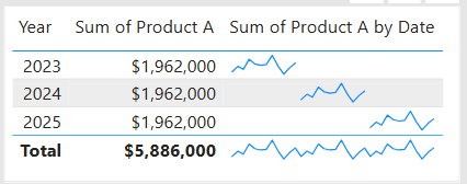
  • Sparklines (Power BI): Miniature line charts embedded in tables or matrices. Ideal for giving quick context without taking up space.

2. Comparing Categories

When to use: To compare values across distinct groups (e.g., sales by region, revenue by product).

Best charts:

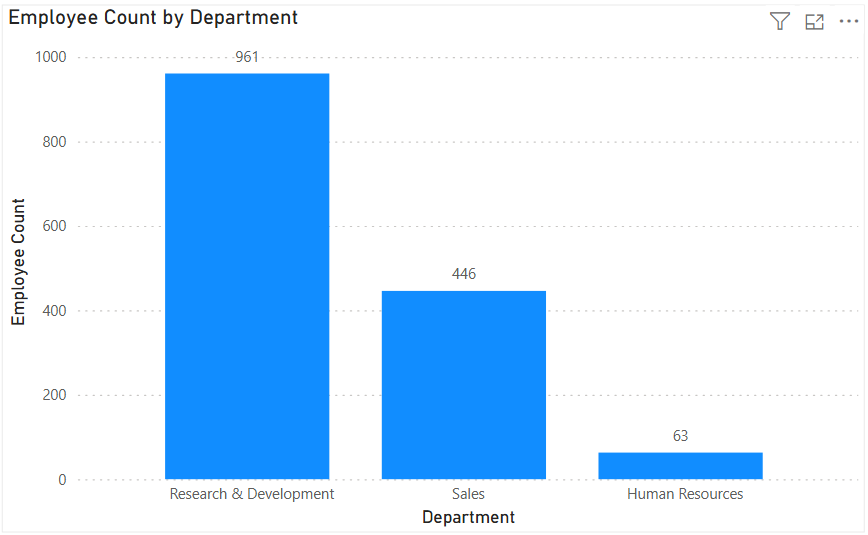
  • Column Chart: Vertical bars for category comparisons. Good when categories are on the horizontal axis.
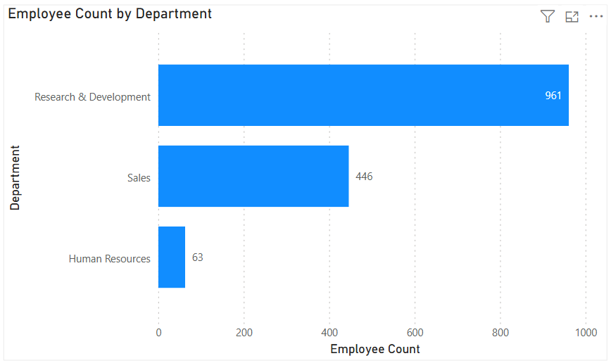
  • Bar Chart: Horizontal bars—useful when category names are long or when ranking items. Is usually a better choice than the column chart when there are many values.
  • Stacked Column/Bar Chart: Show category totals and subcategories in one view. Works for proportional breakdowns, but can get hard to compare across categories.

3. Understanding Relationships

When to use: To see whether two measures are related (e.g., advertising spend vs. sales revenue).

Best charts:

  • Scatter Chart: Plots data points across two axes. Useful for correlation analysis. Add a third variable with bubble size or color to generate more insights. This chart can also be useful for identifying anomalies/outliers in the data.
  • Line & Scatter Combination: Power BI lets you overlay a line for trend direction while keeping the scatter points.
  • Line & Bar/Column Chart Combination: Power BI offers some of these combination charts also to allow you to relate your comparison measures to your trend measures.

4. Highlighting Key Metrics

Sometimes you don’t need a chart—you just want a single number to stand out. These types of visuals are great for high-level executive dashboards, or for the summary page of dashboards in general.

Best visuals in Power BI:

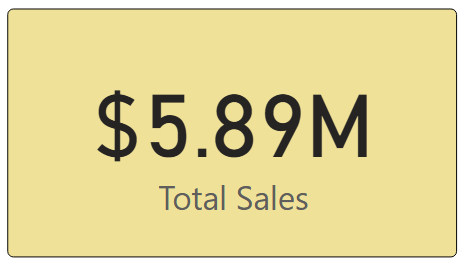
  • Card Visual: Displays one value clearly, like Total Sales.
  • KPI Visual: Adds target context and status indicator (e.g., actual vs. goal).
  • Gauge Visual: Circular representation of progress toward a goal—best for showing percentages or progress to target. For example, Performance Rating score shown on the scale of the goal.

5. Distribution Analysis

When to use: To see how data is spread across categories or ranges.

Best charts:

  • Column/Bar Chart with bins: Useful for creating histograms in Power BI.
  • Box-and-Whisker Chart (custom visual): Shows median, quartiles, and outliers.
  • Pie/Donut Charts: While often overused, they can be effective for showing composition when categories are few (ideally 3–5). For example, show the number and percentage of employees in each department.

6. Spotting Problem Areas

When to use: To identify anomalies or areas needing attention across a large dataset.

Best charts:

  • Heatmap: A table where color intensity represents value magnitude. Excellent for finding hot spots or gaps. This can be implemented in Power BI by using a Matrix visual with conditional formatting in Power BI.
  • Treemap: Breaks data into rectangles sized by value—helpful for hierarchical comparisons and for easily identifying the major components of the whole.

7. Detail-Level Exploration

When to use: To dive into raw data while keeping formatting and hierarchy.

Best visuals:

  • Table: Shows granular row-level data. Best for detail reporting.
  • Matrix: Adds pivot-table–like functionality with rows, columns, and drill-down. Often combined with conditional formatting and sparklines for added insight.

8. Part-to-Whole Analysis

When to use: To see how individual parts contribute to a total.

Best charts:

  • Stacked Charts: Show both totals and category breakdowns.
  • 100% Stacked Charts: Normalize totals so comparisons are by percentage share.
  • Treemap: Visualizes hierarchical data contributions in space-efficient blocks.

Quick Reference: Which Chart to Use?

ScenarioBest Visuals
Tracking trends, forecasting trendsLine, Area, Sparklines
Comparing categoriesColumn, Bar, Stacked
Showing relationshipsScatter, Line + Scatter, Line + Column/Bar
Highlighting metricsCard, KPI, Gauge
Analyzing distributionsHistogram (columns with bins), Box & Whisker, Pie/Donut (for few categories)
Identifying problem areasHeatmap (Matrix with colors), Treemap, Scatter
Exploring detail dataTable, Matrix
Showing part-to-wholeStacked Column/Bar, 100% Stacked, Treemap, Pie/Donut

The below graphic shows the visualization types available in Power BI. You can also import additional visuals by clicking the “3-dots” (get more visuals) at the bottom of the visualization icons.

Summary

Power BI, and other BI/analytics tools, offers a rich set of visuals, each designed to represent data in a way that suits a specific set of analytical needs. The key is to match the chart type with the story you want the data to tell. Whether you’re showing a simple KPI, uncovering trends, or surfacing problem areas, choosing the right chart ensures your insights are clear, actionable, and impactful. In addition, based on your scenario, it can also be beneficial to get feedback from the user population on what other visuals they might find useful or what other ways they would they like to see the data.

Thanks for reading! And good luck on your data journey!

Understanding Microsoft Fabric Shortcuts

Microsoft Fabric is a central platform for data and analytics, and one of its powerful features that supports it being an all-in-one platform is Shortcuts. Shortcuts provide a simple way to unify data across multiple locations without duplicating or moving it. This is a big deal because it saves a LOT of time and effort that is usually involved in moving data around.

What Are Shortcuts?

Shortcuts are references (or “pointers”) to data that resides in another storage location. Instead of copying the data into Fabric, a shortcut lets you access and query it as if it were stored locally.

This is especially valuable in today’s data landscape, where data often spans OneLake, Azure Data Lake Storage (ADLS), Amazon S3, or other environments.

Types of Shortcuts

There are 2 types of shortcuts: table shortcuts and file shortcuts

  1. Table Shortcuts
    • Point to existing tables in other Fabric workspaces or external sources.
    • Allow you to query and analyze the table without physically moving it.
  2. File Shortcuts
    • Point to files (e.g., Parquet, CSV, Delta Lake) stored in OneLake or other supported storage systems.
    • Useful for scenarios where files are your system of record, but you want to use them in Fabric experiences like Power BI, Data Engineering, or Data Science.

Benefits of Shortcuts

Shortcuts is a really useful feature, and here are some of its benefits:

  • No Data Duplication: Saves storage costs and avoids data sprawl.
  • Single Source of Truth: Data stays in its original location while being usable across Fabric.
  • Speed and Efficiency: Query and analyze external data in place, without lengthy ETL processes.
  • Flexibility: Works across different storage platforms and Fabric workspaces.

How and Where Shortcuts Can Be Created

  • In OneLake: You can create shortcuts directly in OneLake to link to data from ADLS Gen2, Amazon S3, or other OneLake workspaces.
  • In Fabric Experiences: Whether working in Data Engineering, Data Science, Real-Time Analytics, or Power BI, shortcuts can be created in lakehouses or KQL (Kusto Query Language) databases, and you can use them directly as data in OneLake. Any Fabric service will be able to use them without copying data from the data source.
  • In Workspaces: Shortcuts make it possible to connect across lakehouses stored in different workspaces, breaking down silos within an organization. The shortcuts can be generated from a lakehouse, warehouse, or KQL database.
  • Note that warehouses do not support the creation of shortcuts. However, you can query data stored within other warehouses and lakehouses.

How Shortcuts Can Be Used

  • Cross-Workspace Data Access: Analysts can query data in another team’s workspace without requesting a copy.
  • Data Virtualization: Data scientists can work with files stored in ADLS without having to move them into Fabric.
  • BI and Reporting: Power BI models can use shortcuts to reference external files or tables, enabling consistent reporting without duplication.
  • ETL Simplification: Instead of moving raw files into Fabric, engineers can create shortcuts and build transformations directly on the source.

Common Scenarios

  • A finance team wants to build Power BI reports on data stored by the operations team without moving the data.
  • A data scientist needs access to parquet files in Amazon S3 but prefers to analyze them within Fabric.
  • A company with multiple Fabric workspaces wants to centralize access to shared reference data (like customer or product master data) without replication.

In summary: Microsoft Fabric Shortcuts simplify data access across locations and workspaces. Whether table-based or file-based, they allow organizations to unify data without duplication, streamline analytics, and improve collaboration.

Here is a link to the Microsoft Learn OneLake documentation about Shortcuts. From there you will be able to explore all the Shortcut topics shown in the image below:

Thanks for reading! I hope you found this information useful.

Mastering the SWITCH Function in Power BI DAX – includes usage and code examples

When building measures and calculated columns in Power BI, we often face situations where we need to evaluate multiple possible outcomes and return different results based on conditions. While IF statements can handle this, they can become cumbersome, confusing, and hard to read when there are many branches.

The SWITCH function in DAX is a cleaner, more efficient alternative for handling multiple condition checks. Let’s take a look.

SWITCH Function Signature

The basic DAX syntax of the SWITCH function is:

SWITCH(<expression>,
       <value1>, <result1>,
       <value2>, <result2>,
       ...,
       [<else>])
  • <expression> – The value or expression you want to evaluate once.
  • <valueN> – A possible value that the expression could equal.
  • <resultN> – The result to return if the expression equals the corresponding <valueN>.
  • [<else>] – (Optional) The default result if none of the value-result pairs match.

Note: the <expression> is evaluated once and compared against multiple <value> options in sequence until a match is found.

Example 1 – Basic SWITCH Usage

Suppose we have a Customer[Category] column containing numeric codes:

  • 1 = “Bronze”
  • 2 = “Silver”
  • 3 = “Gold”

We can translate these codes into readable labels using SWITCH as in the following DAX code example:

Customer Category Label =
SWITCH(Customer[Category],
       1, "Bronze",
       2, "Silver",
       3, "Gold",
       "Unknown"
      )

Explanation:
– The Customer[Category] column is evaluated once.
– If it equals 1, "Bronze" is returned; if 2, "Silver"; if 3, "Gold".
– Otherwise, "Unknown" is returned.

Example 2 – Multiple Match Checks

If we wanted to calculate a commission rate based on a sales tier:

Commission Rate =
SWITCH(Sales[SalesTier],
       "Low", 0.02,
       "Medium", 0.05,
       "High", 0.08,
       0
)

Explanation:
– The Sales[SalesTier] column is evaluated once.
– If it equals "Low", 0.02 is returned; if "Medium", 0.05; if "High", 0.08.
– Otherwise, 0 is returned.

The SWITCH TRUE Pattern

This is a really cool and handy usage of the function. Sometimes, we don’t have a single value to compare against. Instead, we want to evaluate different logical conditions. In these cases, we can use the SWITCH TRUE pattern, which works like multiple IF statements but is much cleaner.

DAX Syntax:

SWITCH( TRUE(),
<condition1>, <result1>,
<condition2>, <result2>,
...,
[<else>])

Here, TRUE() acts as the <expression>. Each <condition> is a Boolean expression that returns TRUE or FALSE. The function returns the corresponding result of the first condition that evaluates to TRUE.

Example 3 – SWITCH TRUE for Ranges

Suppose we want to grade students based on their score:

Grade =
SWITCH(TRUE(),
Scores[Score] >= 90, "A",
Scores[Score] >= 80, "B",
Scores[Score] >= 70, "C",
Scores[Score] >= 60, "D",
"F"
)

Explanation:
– Each Scores[Score] comparison statement is evaluated in order from top to bottom, and returns the first match.
– If Scores[Score] >= 90, “A” is returned; if Scores[Score] >= 80, “B”; if Scores[Score] >= 70, “C”, if Scores[Score] >= 60, “D”
– Otherwise, “F” is returned.

Note: Other more complex conditions, such as ones using OR and AND logic or including complex calculations, can be used.

Why SWITCH is such a great, clean, easy to use function:

  • No nested IFs.
  • Each condition is independent.
  • Easy to add or modify conditions.

When to Use SWITCH Instead of IF

While IF can achieve the same results, SWITCH has several advantages:

  1. Readability – SWITCH structures conditions in a clear, top-to-bottom list.
  2. Maintainability – Easier to add, remove, or change cases without dealing with messy nested parentheses.
  3. Performance – In some cases, SWITCH can be more efficient because the expression (in the basic form) is evaluated once, not multiple times as with nested IF statements.
  4. Logical Branching – The SWITCH TRUE pattern handles complex conditions without deep nesting.

Example 4 – IF vs. SWITCH

Let’s take a look at a comparison example:

IF Version:
Category Label =
IF(Customer[Category] = 1, "Bronze",
IF(Customer[Category] = 2, "Silver",
IF(Customer[Category] = 3, "Gold", "Unknown")
)
)

SWITCH Version:
Category Label =
SWITCH(Customer[Category],
1, "Bronze",
2, "Silver",
3, "Gold",
"Unknown"
)

Result: As you can see, the SWITCH version is shorter, easier to read, less error-prone, and easier to maintain.

Key Takeaways

  • Use basic SWITCH when comparing one expression to multiple possible values.
  • Use SWITCH TRUE when checking multiple conditions or ranges.
  • SWITCH often results in cleaner, more maintainable DAX than deeply nested IF statements.
  • Always include a default (else) value to handle unexpected cases.

Thanks for reading and I hope you found this useful.

Understanding UNION, INTERSECT, and EXCEPT in Power BI DAX

When working with data in Power BI, it’s common to need to combine, compare, or filter tables based on their rows. DAX provides three powerful table / set functions for this: UNION, INTERSECT, and EXCEPT.

These functions are especially useful in advanced calculations, comparative analysis, and custom table creation in reports. If you have used these functions in SQL, the concepts here will be familiar.

Sample Dataset

We’ll use the following two tables throughout our examples:

Table: Sales_2024

The above table (Sales_2024) was created using the following DAX code utilizing the DATATABLE function (or you could enter the data directly using the Enter Data feature in Power BI):

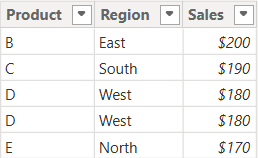
Table: Sales_2025

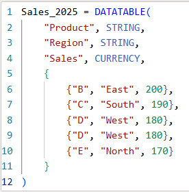
The above table (Sales_2025) was created using the following DAX code utilizing the DATATABLE function (or you could enter the data directly using the Enter Data feature in Power BI):

Now that we have our two test tables, we can now use them to explore the 3 table / set functions – Union, Intersect, and Except.

1. UNION – Combine Rows from Multiple Tables

The UNION function returns all rows from both tables, including duplicates. It requires the same number of columns and compatible data types in corresponding columns in the the tables being UNION’ed. The column names do not have to match, but the number of columns and datatypes need to match.

DAX Syntax:

UNION(<Table1>, <Table2>)

For our example, here is the syntax and resulting dataset:

UnionTable = UNION(Sales_2024, Sales_2025)

As you can see, the UNION returns all rows from both tables, including duplicates.

If you were to reverse the order of the tables (in the function call), the result remains the same (as shown below):

To remove duplicates, you can wrap the UNION inside a DISTINCT() function call, as shown below:

2. INTERSECT – Returns Rows Present in Both Tables

The INTERSECT function returns only the rows that appear in both tables (based on exact matches across all columns).

DAX Syntax:

INTERSECT(<Table1>, <Table2>)

For our example, here is the syntax and resulting dataset:

IntersectTable = INTERSECT(Sales_2024, Sales_2025)

Only the rows in Sales_2024 that are also found in Sales_2025 are returned.

If you were to reverse the order of the tables, you would get the following result:

IntersectTableReverse = INTERSECT(Sales_2025, Sales_2024)

In this case, it returns only the rows in Sales_2025 that are also found in Sales_2024. Since the record with “D – West – $180” exists twice in Sales_2025, and also exists in Sales_2024, then both records are returned. So, while it might not be relevant for all datasets, order does matter when using INTERSECT.

3. EXCEPT – Returns Rows in One Table but Not the Other

The EXCEPT function returns rows from the first table that do not exist in the second.

DAX Syntax:

EXCEPT(<Table1>, <Table2>)

For our example, here is the syntax and resulting dataset:

ExceptTable = EXCEPT(Sales_2024, Sales_2025)

Only the rows in Sales_2024 that are not in Sales_2025 are returned.

If you were to reverse the order of the tables, you would get the following result:

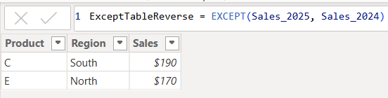
ExceptTableReverse = EXCEPT(Sales_2025, Sales_2024)

Only the rows in Sales_2025 that are not in Sales_2024 are returned. Therefore, as you have seen, since it pulls data from the first table that does not exist in the second, order does matter when using EXCEPT.

Comparison table summarizing the 3 functions:

FunctionUNIONINTERSECTEXCEPT
Purpose & OutputReturns all rows from both tablesReturns rows that appear in both tables (i.e., rows that match across all columns in both tables)Returns rows from the first table that do not exist in the second
Match CriteriaColumn position (number of columns) and datatypesColumn position (number of columns) and datatypes and valuesColumn position (number of columns) and datatypes must match and values must not match
Order Sensitivityorder does not matterorder matters if you want duplicates returned when they exist in the first tableorder matters
Duplicate HandlingKeeps duplicates. They can be removed by using DISTINCT()Returns duplicates only if they exist in the first tableReturns duplicates only if they exist in the first table

Additional Notes for your consideration:

  • Column Names: Only the column names from the first table are kept; the second table’s columns must match in count and data type.
  • Performance: On large datasets, these functions can be expensive, so you should consider filtering the data before using them.
  • Case Sensitivity: String comparisons are generally case-insensitive in DAX.
  • Real-World Use Cases:
    • UNION – Combining a historical dataset and a current dataset for analysis.
    • INTERSECT – Finding products sold in both years.
    • EXCEPT – Identifying products discontinued or newly introduced.

Thanks for reading!

Data Cleaning methods

Data cleaning is an essential step in the data preprocessing pipeline when preparing data for analytics or data science. It involves identifying and correcting or removing errors, inconsistencies, and inaccuracies in the dataset to improve its quality and reliability. It is essential that data is cleaned before being used in analyses, reporting, development or integration. Here are some common data cleaning methods:

Handling missing values:

  • Delete rows or columns with a high percentage of missing values if they don’t contribute significantly to the analysis.
  • Impute missing values by replacing them with a statistical measure such as mean, median, mode, or using more advanced techniques like regression imputation or k-nearest neighbors imputation.

Handling categorical variables:

  • Encode categorical variables into numerical representations using techniques like one-hot encoding, label encoding, or target encoding.

Removing duplicates:

  • Identify and remove duplicate records based on one or more key variables.
  • Be cautious when removing duplicates, as sometimes duplicated entries may be valid and intentional.

Handling outliers:

  • Identify outliers using statistical methods like z-scores, box plots, or domain knowledge.
  • Decide whether to remove outliers or transform them based on the nature of the data and the analysis goals.

Correcting inconsistent data:

  • Standardize data formats: Convert data into a consistent format (e.g., converting dates to a specific format).
  • Resolve inconsistencies: Identify and correct inconsistent values (e.g., correcting misspelled words, merging similar categories).

Dealing with irrelevant or redundant features:

  • Remove irrelevant features that do not contribute to the analysis or prediction task.
  • Identify and handle redundant features that provide similar information to avoid multicollinearity issues.
Data normalization or scaling:

  • Normalize numerical features to a common scale (e.g., min-max scaling or z-score normalization) to prevent certain features from dominating the analysis due to their larger magnitudes.

Data integrity issues:

Finally, you need to address data integrity issues.

  • Check for data integrity problems such as inconsistent data types, incorrect data ranges, or violations of business rules.
  • Resolve integrity issues by correcting or removing problematic data.

It’s important to note that the specific data cleaning methods that need to be applied to a dataset will vary depending on the nature of the dataset, the analysis goals, and domain knowledge. It’s recommended to thoroughly understand the data and consult with domain experts when preparing to perform data cleaning tasks.

Transpose vs. Pivot vs. Unpivot in Power BI

In this post, I will quickly show how to perform 3 key transformations in Power BI – Transpose, Pivot, and Unpivot – and what impact they have on the data they are applied to. These transformations are often needed to manipulate the original data to get it into the shape needed to create the Power BI model and reports. We will use a simple example so that you can see clearly the effect of each transformation.

This is the original dataset – Student Grades:

Transpose

Transpose the data by going to the Transform ribbon and clicking “Transpose”.

This is what the data looks like after the Transpose transformation is applied. The rows are converted into columns, and the columns are converted into rows. Default headers / column names are applied.

Pivot Column

Starting with the original dataset, we will now Pivot the dataset. Go to Transform ribbon, click on “Pivot Column”.

The Pivot Column dialog opens. As noted, it will use the values in the Names column to create new columns, and will use the Score column as the Values Column.

This is what the data looks like after Pivot is applied as described above. Pivot Column converts the selected Name column values into column headers.

Unpivot Columns

Starting with the original dataset, we will now Unpivot the dataset. First select all 4 name columns by using “Ctrl + Click”.

Then, go to Transform ribbon, click on “Unpivot Columns”. This is what the data looks like after the Unpivot Columns transformation is applied. Unpivot Columns converts the selected columns (the name columns in this case) into a column of values (Attribute) and the column values are stored in the Value column.

Thanks for reading!

Setting a table as a date table in Power BI to be able to use the delivered Time Intelligence functions

It is common to have the need to perform time-driven analysis on your data. For example, you may need to compare this month’s sales with the sales from the same period a year ago or you may need to calculate the number of days between two dates. Power BI provides a set of Time Intelligence functions that make it easy to perform these types of calculations. But to take advantage of the Time Intelligence functions in Power BI, you must have a date table in your Power BI model and to have that you will need to “mark” a table as a date table.

To mark a table as a date table, it must meet the following criteria:

  • It must have a column of data type “Date” or “Date/time”. This will be referred to as the “date column”.
  • The date column must contain unique date values. For example, you cannot have the value “3/1/2022” (or any other date value) listed twice (or more than once) in the table.
  • The date column must not contain BLANKs or NULLs. Only unique date values should be in the table’s date column.
  • The date column must not have any missing dates or gaps in dates. For example, you cannot have 1/1/2022 and then 1/3/2022 and not have 1/2/2022 in the date values.
  • The date column must span full years. Keep in mind that a year isn’t necessarily a calendar year (January-December), but should cover the entire 12 months, such as all dates between July 1, 2022 – June 30, 2023, inclusive. If you have less than one year’s dates in your table, then the range can be less than a year, but there cannot be any gaps. Also,

Once these rules are met, you can then mark the table as the date table. To do this, you can either right-click on the table in the Data pane and select “Mark as date table” (as shown below):

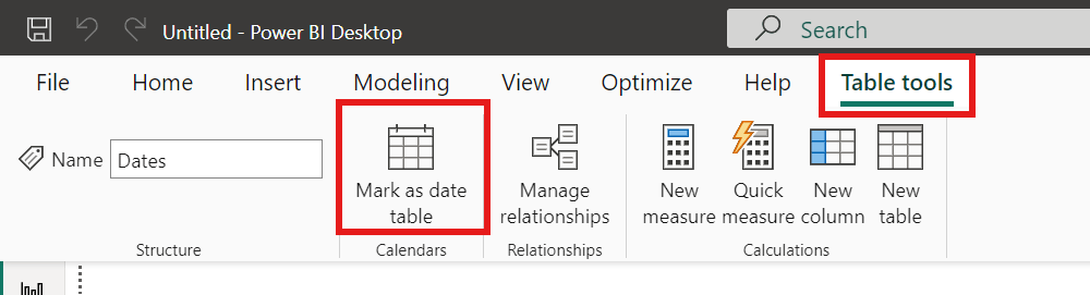
Or with the table selected in the Data pane, from the Table Tools tab, click on the “Mark as date table” icon. This icon will be grayed out if there are no date columns in the table.

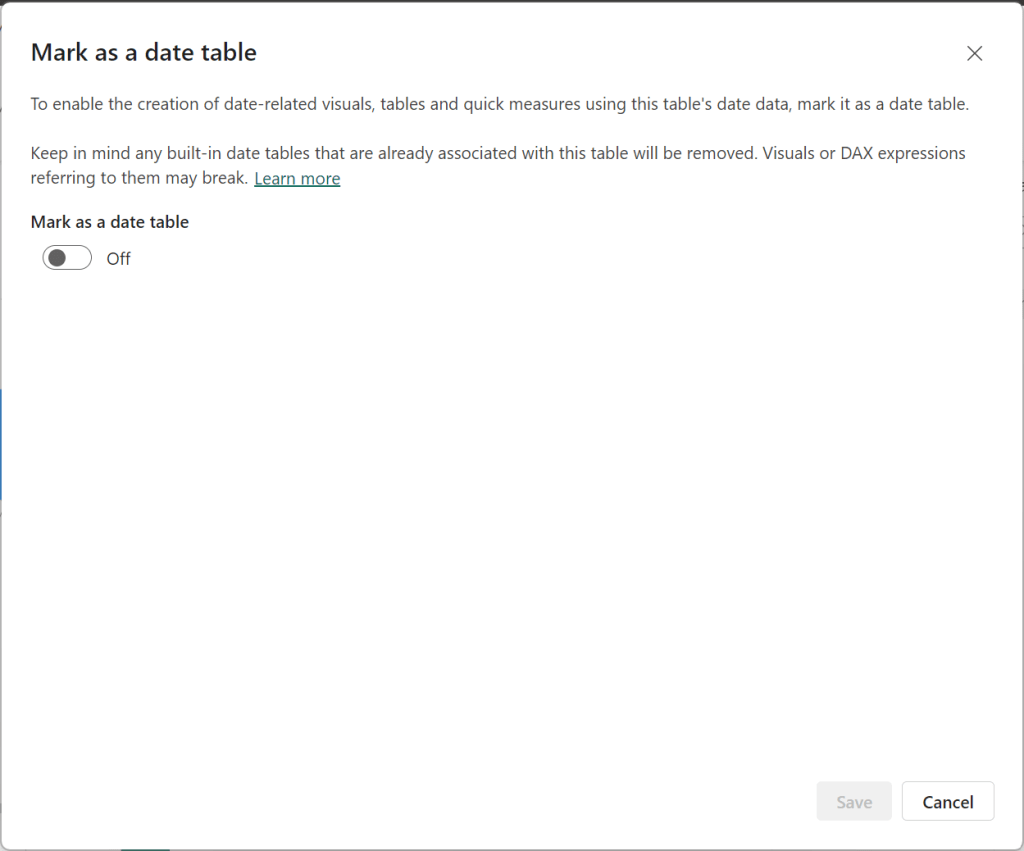
The “Mark as date table” dialog opens (which includes a warning), from which you can turn on the “Mark as date table” flag.

Turn on the flag, and then select / set the date column from the dropdown.

Power BI will then validate your data to make sure all the criteria is met for the chosen column. If you get an error, make the necessary changes and try again.

Thanks for reading!