Like Business Intelligence, the essential purpose of Data Science is to gain knowledge and insights from data. This knowledge can then be used for a variety of purposes – such as, driving more sales, retaining more employees, reducing marketing costs, and saving lives.
This is a continuation of a series of Data Science Fundamentals posts that I will be doing over the next few weeks. In this post, I will be covering Clustering and will include an example to make it more meaningful. A previous post covered Classification. Upcoming posts over the next few days will cover Regression, Matching, and other data science fundamental concepts.
Clustering is similar to Classification, in that, they are both used to categorize and segment data. But Clustering is different from Classification, in that, clustering segments the data into groups (clusters) not previously defined or even known in some cases. Clustering explores the data and finds natural groupings/clusters/classes without any targets (previously defined classes). This is called “unsupervised” segmentation. It clusters the data entities based on some similarity that makes them more like each other than entities in other clusters. Therefore, this is a great first step if information about the data set is unknown.
Clustering: 3 clusters formed (with an outlier)
The Clustering process may yield clusters/groups than can be later used for Classification. Using the defined classes as targets is called “supervised” segmentation. In the diagram to the right, there are 3 clusters that have been formed (red pluses, blue circles, green diamonds).
After a Clustering process is completed, there may be some data entities that are clustered by themselves. In other words, they do not fall into any of the other clusters containing multiple entities. These are classified as outliers. An example of this can be seen in the diagram where there is an outlier in the top-left corner (purple square). Analysis on these outliers can sometimes yield additional insight.
Software such as R and Python provides functions for performing cluster analysis/segmentation on datasets. Future posts will cover these topics along with more details on Clustering.
Over the next 3 months, I will be focusing on Data Science and my next few posts will cover some fundamental topics of Data Science.
The essential purpose of Data Science, like Business Intelligence, is to gain knowledge and insights from data. This knowledge can then be used for a variety of purposes – such as, driving more sales, retaining more employees, reducing marketing costs, and saving lives.
In this post, I will be covering Classification and will include examples to make it more meaningful. Upcoming posts over the next few days will cover Clustering, Regression, Matching, and other data science fundamental concepts.
Classification is the process of using characteristics, features, and attributes of a data entity (such as a person, company, or thing) to determine what class (group or category) it belongs to and assigning it to that class. As an example, demographic data is usually a classification – marital status (married, single, divorced), income bracket (wealthy, middle-class, poor), homeowner status (homeowner or renter), age bracket (old, middle-aged, young), etc.
Shapes are classified by characteristics such as number of sides, length of sides, etc.
When a large amount of data needs to be analyzed, Classification needs to be an automated process. If the classes are not know ahead of time, a process called Clustering can be used on existing data to discover groups that can in some way be used to form the classes.(Clustering will be covered in an upcoming post)
Class Probability Estimation (Scoring) is the process of producing a score that represents the probability of the data entity being in a particular class. As an example, Income Bracket – top 5%.
A few Use Cases and examples of Classification and Class Probably Estimation/Scoring are:
(1) Financial: credit risk – High-Risk, Medium-Risk, Low-Risk, Safe.
A person’s past credit history (or lack of one) will determine their credit score. And their credit score will determine what class of credit risk they fall into, and therefore, will determine if they get the loan, and how favorable the terms of the loan would be.
As an example of Class Probability Estimation (Scoring) for this use case, a person may fall in the Low-Risk class, but their credit score (sometime called FICO score) shows that they are in the low-end of the Low-Risk class making them bordering on Medium-Risk.
(2) Marketing: Marketing offer/promotion interest – Highly likely, Likely, Unlikely
Based on past promotions and those who responded to it, classification can be used to determine the likelihood of a person being interested in a specific marketing offer/promotion. This is known as targeted marketing where specific promotions are sent only to those who will likely be interested, and therefore, different classes/groups may receive different marketing messages from the same company.
As an example of Class Probability Estimation (Scoring) for this use case, a customer or prospect could be scored as 70% Unlikely, or 90% Highly Likely.
(3) Customer Base: Top-customer, Seasonal Customer, Loyal customer, High-Chance of Losing customer, …
A company may use some set of criteria to classify customers into various categories. These categories can be used for various customer-focused efforts, such as marketing, special offers, rewards, and more.
(4) Fraud detection & security: Transaction or Activity occurrence – Highly Unusual, Unusual, Normal
Based on past activity and all other activities as a whole, a person’s activity/transaction can be classified as unusual or normal, and the appropriate actions taken to protect their accounts.
(5) Healthcare:
Data from past health analysis and treatments can be used to classify the level of a patient’s illness, and classify their treatment class. This will then drive the recommended treatment.
(6) Human behavior/Workforce:
Today’s workforce consists of multiple generations (Baby Boomers, GenX, GenY/Millennials, etc) of workers. Generational classification of people based on the period in which they were born is used for marketing purposes, but is also used to help educate a diverse workforce on understanding their team members of different generations and how to work with them.
There are of course many more types of classification and use cases. Feel free to share your use cases.
Your organization may want to have a custom home page or landing page for your OBIEE or OBIA environment. (I will use the term “Landing Page” going forward to not confuse it with the OBIEE delivered “Home Page”). When users log in, they need to be automatically taken to this custom landing page instead of to the delivered OBIEE Home Page.
This post describes some of the reasons you may want a custom landing page, the content that could be on the page, how to automatically navigate users to the page, and security associated with the page.
Why would you want to create a Custom Landing Page? The reasons will vary by organization, but these could be some of the reasons:
Deliver the look and feel that your company or users desire.
Allow for a place that serves as a central location for the content you want to emphasize, in the way you want to display it.
Provide a central place for messages of any kind for your users.
What content will be on this Custom Landing Page? Some of the possibilities are:
Create a page with your custom logos, images, and colors that are in line with your company’s or department’s branding.
A section with messages for your user community. This information could include things such as:
The date/time of the last data load?
The sources of the information displayed on your dashboards
Information about recent dashboard releases
Upcoming downtime
Upcoming events such as user training events
Action needed by the user community
A section that lists links to useful resources, such as:
user’s guides or tutorials
dashboard and report glossary
analysis/report request forms
Security/Access Request forms
general OBI information
A section with Contact Information – containing information about who, what, when, how to contact people for help or information, or how to submit new requests for data/analyses/reports, maybe by functional area, etc.
An area to display your company’s or division’s top key performance indicators (KPIs). These should be limited to just a few – I would say not more than 5 – and they should be relevant company-wide or “OBI user community-wide”.
Links to dashboards. You may create an area or areas of links to various dashboards. Your dashboard list may include many of your dashboards or just a select few that you know are frequently used or that you want to emphasize.
All users that are authorized to use the OBI system will have access to this page. So, maybe BI Consumer role will be provided access.
However, you will need to set security on the sections containing links to dashboards to allow access only to those authorized for the each set of dashboards.
Once your custom landing page is ready, you will then need to set it as the default page for users (or a subset of users). To do this you will need to create an initialization block that sets the PORTALPATH built-in OBI variable to point to the new landing page dashboard page.
One final note … you can have multiple custom landing pages if you desire, for example, a different page for each division or a different page for each major group of users. You would then need to set the PORTALPATH variable based on the user’s profile.
This post describes a scenario for loading data into QlikView from multiple Excel files with similar but different names and a different number of tabs.
Let’s say you need to load multiple Excel files containing information about orders into your QlikView application. These files have different names, and each file may have a different amount of sheets.
For example, you may have several files with Order information from different sources for multiple dates such as:
Let’s say each file has one or more sheets representing regions/divisions – West, Mid-West, North East, and South. Some files may have all 4 region/division sheets, while others may have just one region sheet.
This script is one possible way of loading this data in QlikView using a single script. With some adjustments, this script may also work for Qlik Sense, but I did not test exactly what changes would be needed.
//-----------------------------------------------
// set the errormode so that your script will not fail when one or more of
// the 4 sheets is not found in any particular file
 SET ErrorMode = 0;
OrdersFileData:
 LOAD [CustomerID]  as [Customer ID],
 [OrderID           as [Order Number],
 [OrderDate]        as [Order Date],
 [ShipDate]         as [Ship Date],
 [Notes]            as [Order Notes],
 [Turn around days] as [Turnaround Days],
 'WEST'             as [Division] //identify region/division on all records
 FROM [..DataText Files*Orders*.xlsx] //wildcard allows load from all
                                         //xlsx files with “Orders” in the name
 (ooxml, embedded labels, table is WEST);  //load from the West sheet
CONCATENATE (OrdersFileData) //append data from Midwest sheet from all files
 LOAD [CustomerID]  as [Customer ID],
 [OrderID]          as [Order Number],
 [OrderDate]        as [Order Date],
 [ShipDate]         as [Ship Date],
 [Notes]            as [Order Notes],
 [Turn around days] as [Turnaround Days],
 'MIDWEST'          as [Division]
 FROM [..DataText Files*Orders*.xlsx]
 (ooxml, embedded labels, table is MIDWEST);
CONCATENATE (OrdersFileData) //append data from Northeast sheet from all files
 LOAD [CustomerID] as [Customer ID],
 [OrderID] as [Order Number],
 [OrderDate] as [Order Date],
 [ShipDate] as [Ship Date],
 [Notes] as [Order Notes],
 [Turn around days] as [Turnaround Days],
 'NORTHEAST' as [Division]
 FROM [..DataText Files*Orders*.xlsx]
 (ooxml, embedded labels, table is NORTHEAST);
CONCATENATE (OrdersFileData) //append data from South sheet from all files
 LOAD [CustomerID] as [Customer ID],
 [OrderID] as [Order Number],
 [OrderDate] as [Order Date],
 [ShipDate] as [Ship Date],
 [Notes] as [Order Notes],
 [Turn around days] as [Turnaround Days],
 'SOUTH' as [Division]
 FROM [..DataText Files*Orders*.xlsx]
 (ooxml, embedded labels, table is SOUTH);

STORE OrdersFileData into ..DataQVDsOrdersData.QVD; // if loading to QVD
DROP Table OrdersFileData; //if loading to QVD and not needed in memory
//-----------------------------------------------
Occasionally you may need to check one of your database’s version for the purpose of creating a ticket with the software vendor, for checking compatibility with other software, preparing for upgrades, getting database client software, and other reasons.
Below are commands for identifying the version of your database for a few of the more popular RDBMS’s. Please keep in mind that these may or may not work on your version of database or type of operating system.
ORACLE
SELECT * FROM V$VERSION;
Your output will be something like this …
SQL SERVER
Try one of the following:
Select “Help -> About” from the SQL Server Management Studio menu.
select @@version
You may also connect to the server by using Object Explorer in SQL Server Management Studio. After Object Explorer is connected, it will show the version information in parentheses, together with the user name that is used to connect to the specific instance of SQL Server.
MYSQL
Try one of the following:
shell> mysql –version
mysql> SHOW VARIABLES LIKE ‘%version%’;
mysqladmin version -or- mysqladmin –v
DB2
Try one of the following:
SELECT * FROM TABLE(SYSPROC.ENV_GET_INST_INFO());
SELECT GETVARIABLE(‘SYSIBM.VERSION’) FROM SYSIBM.SYSDUMMY1;
Apache Hadoop, simply termed Hadoop, is an increasingly popular open-source framework for distributed computing. It has had a major impact on the business intelligence / data analytics / data warehousing space, spawning a new practice in this space, referred to as Big Data. Hadoop’s core architecture consists of a storage part known as Hadoop Distributed File System (HDFS) and a processing part called MapReduce. It provides a reliable, scalable, and cost-effective means for storing and processing large data sets, and it does so like no other software frameworks before its time.
It is cost-effective and scalable because it is designed to run on commodity hardware servers that can be scaled from one to hundreds, or even thousands, therefore avoiding the cost of the expensive super-computers (which eventually hits limits). With Hadoop, you are able to add commodity servers as needed without much difficulty at minimal costs.
It is reliable because all the modules in Hadoop are designed with a fundamental assumption that hardware failures will occur and these failures should be automatically handled in software by the Hadoop framework.
Beyond the core components, the Hadoop eco-system has grown to include a number of additional packages that run on top of or alongside the core Hadoop components, including but not limited to, Apache Hive, Apache Pig, Apache HBase, Apache Phoenix, Apache Spark, Apache ZooKeeper, Impala, Apache Flume, Apache Sqoop, Apache Oozie, Apache Storm, Apache Mahout, Ambari, Apache Drill, Tez, and others. This post will serve as a quick look-up for the components of the eco-system to allow you to quickly identify what the components are and understand what they do.
Hadoop component
Component Category
Purpose / Usage
Hadoop
The ecosystem
The core Apache Hadoop framework is composed of the following modules:
Hadoop Common
Hadoop Distributed File System (HDFS)
Hadoop YARN
Hadoop MapReduce
Hadoop Common
Software Libraries shared across the ecosystem
Hadoop Common contains libraries and utilities needed by other Hadoop modules
Hadoop Distributed File System (HDFS)
Distributed Storage
HDFS is a distributed file system that is the foundational storage component of Hadoop and it sits on top of the file system of the commodity hardware that Hadoop runs on. It stores data on these commodity servers and provides high bandwidth and throughput across the cluster of servers.
Hadoop YARN
Resource Management & Scheduling
YARN (which stands for Yet Another Resource Negotiator) is a resource-management platform that manages computing resources in Hadoop clusters and uses them to schedule users’ applications.
Hadoop MapReduce
Distributed Processing
MapReduce is a programming and processing paradigm that pairs with HDFS for large scale data processing.
It is a distributed computational algorithm comprised of a Map() procedure and a Reduce() procedure that pushes computation down to each server in the Hadoop cluster.
The Map procedure performs functions such as filtering and sorting of data; while the Reduce() procedure performs summary / aggregate type operations on the data.
Hive
MapReduce Abstraction / Analysis / Querying
Apache Hive is a data warehouse infrastructure that provides an abstraction layer on top of MapReduce. It provides a SQL-like language called HiveQL and transparently converts queries to MapReduce, Apache Tez, and Apache Spark jobs.
It can handle analysis of large datasets and provides functionality for indexing, data summarization, query, and analysis of the data stored in HDFS or other compatible file systems.
Pig
MapReduce Abstraction / Analysis / Querying
Pig is a functional programming interface that allows you to use a higher level scripting language (called Pig Latin) to create MapReduce code for Hadoop. Pig is similar to PL/SQL and can be extended using UDF’s written in Java, Python and other languages.
It was originally developed to provide analysts an ad-hoc way of creating and executing map-reduce jobs on very large data sets.
Ambari
Monitoring & Management of Clusters
Ambari is a web-based tool for provisioning, managing, and monitoring Apache Hadoop clusters. It includes support for many of the key components of the Hadoop eco-system, such as, Hadoop HDFS, Hadoop MapReduce, Hive, HCatalog, HBase, ZooKeeper, Oozie, Pig and Sqoop.
Ambari also provides a user-friendly dashboard for viewing cluster health and MapReduce, Pig and Hive applications, And it also provides features to diagnose the performance of the various components.
HBase
Storage / database
HBase is a non-relational (NoSQL) distributed, fast, and scalable database that runs on top of HDFS. It is modeled after Google’s Big Table, providing BigTable-like capabilities to Hadoop, and is written in Java.
It provides fault-tolerant storage and retrieval of huge quantities of sparse data – such as top 10 out of 10 billion records or the 0.1% of recrods that are non-zero.
HBase features include compression, and in-memory operation. HBase tables can be used as the input and output for MapReduce jobs run in Hadoop, and are accessed through APIs.
HBase can be integrated with BI and Analytics applications through drivers and through Apache Phoenix’s SQL layer. However, HBase is not a RDBMS replacement.
Hue
Web GUI
Hue is an open-source Web interface for end users that supports Apache Hadoop and its ecosystem.
Hue provides a single interface for the most common Apache Hadoop components with an emphasis on user experience. Its main goal is to have the users make the most of Hadoop without worrying about the underlying complexity or using a command line.
Sqoop
Data Integration
Sqoop, named from a combination of SQL+Hadoop, is an application with a command-line interface that pulls and pushes data from/to relational data sources, to/from Hadoop.
It supports compression, incremental loads of a single table, or a free form SQL query. You can also save jobs which can be run multiple times to perform the incremental loads. Imports can also be used to populate tables in Hive or HBase.
Exports can be used to put data from Hadoop into a relational database.
Several software vendors provide Sqoop-based functionality into their database and BI/analytics products.
Flume
Data Integration
Apache Flume is a distributed service for efficiently collecting, aggregating, and moving large amounts of log data (such as web logs or sensor data) into and out of Hadoop (HDFS).
It features include fault tolerance and a simple extensible data model that supports streaming data flows and allows for online analysis.
Impala
Analysis / Querying
Cloudera Impala is a massively parallel processing, low-latency SQL Query engine that runs on Hadoop and communicates directly with HDFS, bypassing MapReduce.
It allows you to run SQL queries in lower data volume scenarios on data stored in HDFS and HBase, and returns results much quicker than Pig and Hive.
Impala is designed and integrated with Hadoop to use the same file and data formats, metadata, security and resource management frameworks used by MapReduce, Apache Hive, Apache Pig and other Hadoop software, which allows for both large scale data processing and interactive queries to be done on the same system.
Impala is great for data analysts and scientists to perform analytics on data stored in Hadoop via SQL or other business intelligence tools.
Avro
Data Integration
Avro is a data interchange protocol/framework that provides data serialization and de-serialization in a compact binary format.
Its primary use is in Apache Hadoop, where it can provide both a serialization format for persistent data, and a wire format for communication between Hadoop nodes, and from client programs to the Hadoop services.
Storm
Data Integration
Apache Storm is a distributed computation framework, written predominantly in the Clojure programming language that moves streaming data into and out of Hadoop.
It allows for the definition of information sources and manipulations to allow batch, distributed processing of streaming data.
Storm’s architecture acts as a data transformation pipeline. At a very high level the general architecture is similar to a MapReduce job, with the main difference being that data is processed in real-time as opposed to in individual batches.
Oozie
Workflow Builder
Apache Oozie is a server-based workflow scheduling system, built using Java, to manage Hadoop jobs. It chains together MapReduce jobs, and data import/export scripts.
Workflows in Oozie are defined as a collection of control flow and action nodes. Action nodes are the mechanism by which a workflow triggers the execution of a computation/processing task. Oozie provides support for different types of actions including Hadoop MapReduce, HDFS operations, Pig, SSH, and email; and it can be extended to support additional types of actions.
Mahout
Machine Learning
Apache Mahout is a set of libraries for distributed, scalable machine learning; data mining; and mathematical algorithms that run primarily on the Hadoop, and focused primarily in the areas of collaborative filtering, clustering and classification.
Mahout’s core algorithms for clustering, classification and batch based collaborative filtering are implemented on top of Apache Hadoop using the map/reduce paradigm, but is not restricted to Hadoop-based implementations.
ZooKeeper
Coordination
ZooKeeper is a high-performance, high-availability coordination service for distributed applications. It provides a distributed configuration service, synchronization service, and naming registry for large distributed systems.
ZooKeeper is used by open source enterprise search systems like Solr.
Spark
Data Integration, Processing, Machine Learning
Apache Spark sits directly on top of HDFS, bypassing MapReduce, and is a fast, general compute engine for Hadoop. It is said that Spark could eventually replace MapReduce because it provides solutions for everything MapReduce does, plus adds a lot more functionality.
It uses a different paradigm from MapReduce (synonymous to rows vs sets processing in SQL), and uses more in-memory capabilities which makes it typically faster than MapReduce. In contrast to MapReduce’s two-stage disk-based paradigm, Spark’s multi-stage in-memory primitives provides performance up to 100 times faster for certain applications.
Spark is very versatile and provides a simple and expressive programming model that supports a wide range of applications, including ETL, machine learning, stream processing, and graph computation.
Spark requires a cluster manager and supports standalone (native Spark cluster), Hadoop YARN, or Apache Mesos; and also requires a distributed storage system such as Hadoop Distributed File System (HDFS), Cassandra, Amazon S3, or even custom systems; but it does support a pseudo-distributed local mode (for development and testing).
Spark is one of the most active projects in the Apache Software Foundation.
Phoenix
Data Manipulation
Apache Phoenix is a massively parallel, relational database layer on top of noSQL stores such as Apache HBase.
Phoenix provides a JDBC driver that hides the complexities of the noSQL store enabling users to use the familiar SQL to create, delete, and alter SQL tables, views, indexes, and sequences; insert, update, and delete rows singly and in bulk; and query data.
Phoenix compiles queries and other statements into native noSQL store APIs rather than using MapReduce enabling the building of low latency applications on top of noSQL stores.
Cassandra
Storage / database
Apache Cassandra is an open source, scalable, multi-master, high-performance, distributed database management system designed to handle large amounts of data across many commodity servers, providing high availability with no single point of failure.
Cassandra supports clusters spanning multiple datacenters, with asynchronous masterless replication allowing for low latency operations.
Solr
Search
Solr (pronounced “solar”) is an open source enterprise search platform, written in Java, and runs as a standalone full-text search server.
Its features include full-text search, hit highlighting, faceted search, real-time indexing, dynamic clustering, database integration, NoSQL capabilities, and rich document (e.g., Word, PDF) handling. Solr is designed for scalability and Fault tolerance with distributed search and index replication. Solr is a very popular enterprise search engine.
Solr has APIs and a plugin architecture that makes it customizable using various programming languages.
There is the flexibility to root the data being brought in by SQOOP and FLUME directly into SOLR to do indexing on the fly. But you can also tell SOLR to index the data in batches.
MongoDB
Storage / database
MongoDB (from humongous) is an open-source, cross-platform document-oriented, NoSQL database. It uses a JSON-like structure, called BSON, with dynamic schemas which makes the integration of data in certain types of applications easier and faster.
MongoDB is one of the most popular type of database management systems, and is said to be the most popular for document stores.
Kafka
Data Integration
Apache Kafka is an open-source message broker project written in Scala. It provides a unified, high-throughput, low-latency platform for handling real-time data feeds. The design is heavily influenced by transaction logs.
Apache Kafka was originally developed by LinkedIn, and was subsequently open sourced in early 2011.
Accumulo
Storage / database
Apache Accumulo is a data store with a sorted, distributed key/value and, like HBase, is based on the BigTable technology from Google. It is written in Java, and is built on top of Apache Hadoop, Apache ZooKeeper, and Apache Thrift. Accumulo is said to be third most popular NoSQL wide column store behind Apache Cassandra and HBase as of 2015.
Chukwa
Data Integration
Chukwa is a data collection system for managing large distributed systems.
Tez
Processing
Tez is a flexible data-flow programming framework, built on Hadoop YARN, that processes both in batch and interactive modes. It is being adopted by Hive, Pig and other frameworks in the Hadoop ecosystem, and also by other commercial software (e.g. ETL tools), to replace Hadoop MapReduce as the underlying execution engine.
Drill
Processing
Apache Drill is an open-source software framework that supports data-intensive distributed applications for interactive analysis of large-scale datasets, even across multiple data stores, at amazing speed.
It is the open source version of Google’s Dremel system which is available as a service called Google BigQuery, and it supports a variety of NoSQL databases and file systems, including HBase, MongoDB, HDFS, Amazon S3, Azure Blob Storage, local files, and more.
Apache Sentry
Security
Apache Sentry is a system for enforcing fine grained role based authorization to data and metadata stored on a Hadoop cluster.
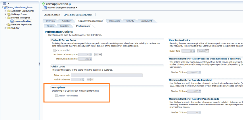
You may want to disable online updates on your OBIEE RPD for performance reasons or because you have a specific development process that prohibits online updates.
To disallow online RPD updates, do the following:
Log into Enterprise Manager. Navigate the tree menu to Business Intelligence -> coreapplication. Click tabs “Capacity Management”, and “Performance”.
Under the RPD Updates section, check the box for “Disallow RPD updates”.
This will prevent online RPD updates for all.
If you want to allow a select group of people to have access to perform online updates, such as a lead developer or administrator, then don’t do the above, but instead provide Administrator role to those that should have the access, and remove it from those that should not (and give them BI Author role for example instead).
Tableau is a leading business intelligence software. Its popularity has grown as a result of its ease of use, awesome visualizations, ability to connect easily to many data sources, its ability to make use of Big Data and Cloud sources, and many other traditional and cutting-edge features.
In this post, I will guide you through the installation of Tableau Desktop 9. It’s pretty simple.
Navigate to where you saved the download and double-click the file (in this example, TableauDesktop-64bit-9-3-4.exe) to execute or right-click the file and select Run as administrator.
Read and accept the license agreement.
Click Install if you want to install with defaults.
Or you may also click Customize to change some default settings. Clicking Customize will bring you to the following dialog.
From here you may change the install directory and check/uncheck options as you see fit. Click Install.
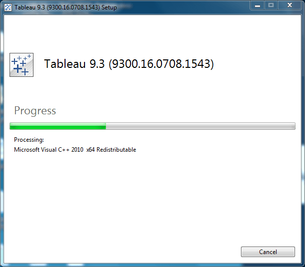
Installation in progress.
Installation is complete. Choose the desired Activation schedule.
You have 14 days from activation to use the product.
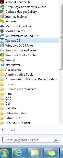
Unless you had unchecked this option, Tableau will be added to your Windows start menu.
We are on Oracle Business Intelligence Applications (OBIA) 7.9.6.3 and had been experiencing performance issues with the SIL_APTransactionFact_DiffManLoad workflow/mapping. We tried a number of things but only had minimal improvements. Eventually, I found a solution for the poor performance on Oracle Support. This change resulted in a drastic improvement of this workflow.
The solution can be found on Oracle Support (http://support.oracle.com – Oracle Doc ID: 1446397.1), but for your convenience I have included the content below. There are other mappings that have a similar problem.
————————————————————————
OBIA 7963: SIL_APTransactionFact_Diffmanload Mapping And Performance Issue (Doc ID 1446397.1)
In this Document
Symptoms
Cause
Solution
Applies to:
Informatica OEM PowerCenter ETL Server – Version 7.9.6.3 [AN 1900] and later Information in this document applies to any platform.
Symptoms
The OBIEE application (7.9.6.3) ETL task “SIL_APTransactionFact_DiffManLoad” has run over 68 hours during full load execution.
Cause
The size of these columns (DOC_HEADER_TEXT and LINE_ITEM_TEXT ) in DAC is 255 (except AP where its 1020 in DAC and Infa). But in Informatica the size for these two columns is 1020. Ideally it should be 255. This is a known performance issue.
The cause of the problem has been identified in unpublished Bug 12412793- PSR: B16 INCREMENTAL: SIL_GLREVENUEFACT,
Solution
Below are the steps you will follow to modify the size of the fields in the lookup.
Take a backup of existing Lookups ( LKP_W_AP_XACT_F and LKP_W_AR_XACT_F ).
Login to Informatica Designer >Transformations
Open the lookup and modify the size of the fields. The port lengths for the DOC_HEADER_TEXT and LINE_ITEM_TEXT were changed to 255 .
Save the changes
Rerun the test and confirm the performance issue is resolved and migrate the changes in PROD.
You will get to information such as that shown in the screenshot below …
Click on “System requirements” and “Browser support” to get information on system and browser requirements before starting the installation. System requirements will show operating system, processor, memory and disk space requirements among other things. And browser support will specify the browsers required for each supported OS.
Click on “Obtaining the setup file” to access the installation file
Click “Download Qlik Sense Desktop”
Click the FREE DOWNLOAD button
After the download is complete, navigate to the folder where you saved the file.
Run the setup executable (Qlik_Sense_Desktop_setup.exe) by double-clicking on it. In some cases, it is best to right-click on the setup executable, and “Run as administrator”.
Click on “Accept and Install” to acknowledge that Microsoft .NET Framework will be installed and continue to installation process.
Close all other applications, and click Install.
Accept the license agreement and click Next.
If desired, check “Create desktop shortcuts”. Click Install.
The installation is complete. Click Finish.
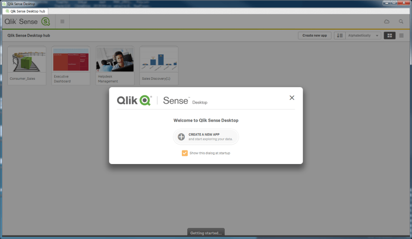
Either from the Windows menu or from the desktop icon, launch Qlik Sense.
You are ready to start using Qlik Sense 3.0. It’s that simple.
If you get an error message that reads … “An error occurred. The service did not respond or could not process the request.” … then read the article on this site that addresses that issue to see how to resolve.
Information and resources for the data professionals' community