When working with data in Power BI, it’s common to need to combine, compare, or filter tables based on their rows. DAX provides three powerful table / set functions for this: UNION, INTERSECT, and EXCEPT.
These functions are especially useful in advanced calculations, comparative analysis, and custom table creation in reports. If you have used these functions in SQL, the concepts here will be familiar.
Sample Dataset
We’ll use the following two tables throughout our examples:
Table: Sales_2024

The above table (Sales_2024) was created using the following DAX code utilizing the DATATABLE function (or you could enter the data directly using the Enter Data feature in Power BI):

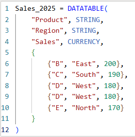
Table: Sales_2025
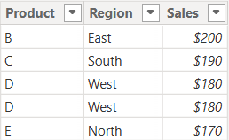
The above table (Sales_2025) was created using the following DAX code utilizing the DATATABLE function (or you could enter the data directly using the Enter Data feature in Power BI):
Now that we have our two test tables, we can now use them to explore the 3 table / set functions – Union, Intersect, and Except.
1. UNION – Combine Rows from Multiple Tables
The UNION function returns all rows from both tables, including duplicates. It requires the same number of columns and compatible data types in corresponding columns in the the tables being UNION’ed. The column names do not have to match, but the number of columns and datatypes need to match.
DAX Syntax:
UNION(<Table1>, <Table2>)
For our example, here is the syntax and resulting dataset:
UnionTable = UNION(Sales_2024, Sales_2025)

As you can see, the UNION returns all rows from both tables, including duplicates.
If you were to reverse the order of the tables (in the function call), the result remains the same (as shown below):

To remove duplicates, you can wrap the UNION inside a DISTINCT() function call, as shown below:

2. INTERSECT – Returns Rows Present in Both Tables
The INTERSECT function returns only the rows that appear in both tables (based on exact matches across all columns).
DAX Syntax:
INTERSECT(<Table1>, <Table2>)
For our example, here is the syntax and resulting dataset:
IntersectTable = INTERSECT(Sales_2024, Sales_2025)
Only the rows in Sales_2024 that are also found in Sales_2025 are returned.
If you were to reverse the order of the tables, you would get the following result:
IntersectTableReverse = INTERSECT(Sales_2025, Sales_2024)

In this case, it returns only the rows in Sales_2025 that are also found in Sales_2024. Since the record with “D – West – $180” exists twice in Sales_2025, and also exists in Sales_2024, then both records are returned. So, while it might not be relevant for all datasets, order does matter when using INTERSECT.
3. EXCEPT – Returns Rows in One Table but Not the Other
The EXCEPT function returns rows from the first table that do not exist in the second.
DAX Syntax:
EXCEPT(<Table1>, <Table2>)
For our example, here is the syntax and resulting dataset:
ExceptTable = EXCEPT(Sales_2024, Sales_2025)
Only the rows in Sales_2024 that are not in Sales_2025 are returned.
If you were to reverse the order of the tables, you would get the following result:
ExceptTableReverse = EXCEPT(Sales_2025, Sales_2024)
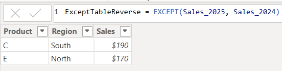
Only the rows in Sales_2025 that are not in Sales_2024 are returned. Therefore, as you have seen, since it pulls data from the first table that does not exist in the second, order does matter when using EXCEPT.
Comparison table summarizing the 3 functions:
| Function | UNION | INTERSECT | EXCEPT |
| Purpose & Output | Returns all rows from both tables | Returns rows that appear in both tables (i.e., rows that match across all columns in both tables) | Returns rows from the first table that do not exist in the second |
| Match Criteria | Column position (number of columns) and datatypes | Column position (number of columns) and datatypes and values | Column position (number of columns) and datatypes must match and values must not match |
| Order Sensitivity | order does not matter | order matters if you want duplicates returned when they exist in the first table | order matters |
| Duplicate Handling | Keeps duplicates. They can be removed by using DISTINCT() | Returns duplicates only if they exist in the first table | Returns duplicates only if they exist in the first table |
Additional Notes for your consideration:
- Column Names: Only the column names from the first table are kept; the second table’s columns must match in count and data type.
- Performance: On large datasets, these functions can be expensive, so you should consider filtering the data before using them.
- Case Sensitivity: String comparisons are generally case-insensitive in DAX.
- Real-World Use Cases:
UNION– Combining a historical dataset and a current dataset for analysis.INTERSECT– Finding products sold in both years.EXCEPT– Identifying products discontinued or newly introduced.
Thanks for reading!


