Category: Data Wrangling

Convert Semi-Structured Data to a Table (PL-300 Exam Prep)

This post is a part of the PL-300: Microsoft Power BI Data Analyst Exam Prep Hub; and this topic falls under these sections:
Prepare the data (25–30%)
--> Transform and load the data
--> Convert Semi-Structured Data to a Table


Note that there are 10 practice questions (with answers and explanations) for each section to help you solidify your knowledge of the material. Also, there are 2 practice tests with 60 questions each available on the hub below the exam topics section.

In real-world analytics, data rarely arrives in a perfectly tabular format. Instead, analysts often work with semi-structured data, such as JSON files, XML documents, nested records, lists, or poorly formatted spreadsheets.

For the PL-300: Microsoft Power BI Data Analyst exam, Microsoft expects you to understand how to convert semi-structured data into a clean, tabular format using Power Query so it can be modeled, related, and analyzed effectively.


What Is Semi-Structured Data?

Semi-structured data does not follow a strict row-and-column structure but still contains identifiable elements and hierarchy.

Common examples include:

  • JSON files (nested objects and arrays)
  • XML files
  • API responses
  • Excel sheets with nested headers or inconsistent layouts
  • Columns containing records or lists in Power Query

Exam insight: The exam does not focus on file formats alone — it focuses on recognizing non-tabular structures and flattening them correctly.


Where This Happens in Power BI

All semi-structured data transformations are performed in Power Query Editor, typically using:

  • Convert to Table
  • Expand (↔ icon) for records and lists
  • Split Column
  • Transpose
  • Fill Down / Fill Up
  • Promote Headers
  • Remove Blank Rows / Columns

Common Semi-Structured Scenarios (Exam Favorites)

1. JSON and API Data

When loading JSON or API data, Power Query often creates columns containing:

  • Records (objects)
  • Lists (arrays)

These must be expanded to expose fields and values.

Example:

  • Column contains a Record → Expand to columns
  • Column contains a List → Convert to Table, then expand

2. Columns Containing Lists

A column may contain multiple values per row stored as a list.

Solution path:

  • Convert list to table
  • Expand values into rows
  • Rename columns

Exam tip: Lists usually become rows, while records usually become columns.


3. Nested Records

Nested records appear as a single column with structured fields inside.

Solution:

  • Expand the record
  • Select required fields
  • Remove unnecessary nested columns

4. Poorly Formatted Excel Sheets

Common examples:

  • Headers spread across multiple rows
  • Values grouped by section
  • Blank rows separating logical blocks

Typical transformation sequence:

  1. Remove blank rows
  2. Fill down headers
  3. Transpose if needed
  4. Promote headers
  5. Rename columns

Key Power Query Actions for This Topic

Convert to Table

Used when:

  • Data is stored as a list
  • JSON arrays need flattening
  • You need row-level structure

Expand Columns

Used when:

  • Columns contain records or nested tables
  • You want to expose attributes as individual columns

You can:

  • Expand all fields
  • Select specific fields
  • Avoid prefixing column names (important for clean models)

Promote Headers

Often used after:

  • Transposing
  • Importing CSV or Excel files with headers in the first row

Fill Down

Used when:

  • Headers or categories appear once but apply to multiple rows
  • Semi-structured data uses grouping instead of repetition

Impact on the Data Model

Converting semi-structured data properly:

  • Enables relationships to be created
  • Allows DAX measures to work correctly
  • Prevents ambiguous or unusable columns
  • Improves model usability and performance

Improper conversion can lead to:

  • Duplicate values
  • Inconsistent grain
  • Broken relationships
  • Confusing field names

Exam insight: Microsoft expects you to shape data before loading it into the model.


Common Mistakes (Often Tested)

❌ Expanding Too Early

Expanding before cleaning can introduce nulls, errors, or duplicated values.


❌ Keeping Nested Structures

Leaving lists or records unexpanded results in columns that cannot be analyzed.


❌ Forgetting to Promote Headers

Failing to promote headers leads to generic column names (Column1, Column2), which affects clarity and modeling.


❌ Mixing Granularity

Expanding nested data without understanding grain can create duplicated facts.


Best Practices for PL-300 Candidates

  • Inspect column types (Record vs List) before expanding
  • Expand only required fields
  • Rename columns immediately after expansion
  • Normalize data before modeling
  • Know when NOT to expand (e.g., reference tables or metadata)
  • Validate row counts after conversion

How This Appears on the PL-300 Exam

Expect scenario-based questions like:

  • A JSON file contains nested arrays — what transformation is required to analyze it?
  • An API response loads as a list — how do you convert it to rows?
  • A column contains records — how do you expose the attributes for reporting?
  • What step is required before creating relationships?

Correct answers focus on Power Query transformations, not DAX.


Quick Decision Guide

Data ShapeRecommended Action
JSON listConvert to Table
Record columnExpand
Nested list inside recordConvert → Expand
Headers in rowsTranspose + Promote Headers
Grouped labelsFill Down

Final Exam Takeaways

  • Semi-structured data must be flattened before modeling
  • Power Query is the correct place to perform these transformations
  • Understand the difference between lists, records, and tables
  • The exam tests recognition and decision-making, not syntax memorization

Practice Questions

Go to the Practice Exam Questions for this topic.

How to Perform a Safe DIVIDE in Power BI (DAX and Power Query)

Division is a common operation in Power BI, but it can cause errors when the divisor is zero. Both DAX and Power Query provide built-in ways to handle these scenarios safely.

Safe DIVIDE in DAX

In DAX, the DIVIDE function is the recommended approach. Its syntax is:

DIVIDE(numerator, divisor [, alternateResult])

If the divisor is zero (or BLANK), the function returns the optional alternateResult; otherwise, it performs the division normally.

Examples:

  • DIVIDE(10, 2)5
  • DIVIDE(10, 0)BLANK
  • DIVIDE(10, 0, 0)0

This makes DIVIDE safer and cleaner than using conditional logic.

Safe DIVIDE in Power Query

In Power Query (M language), you can use the try … otherwise expression to handle divide-by-zero errors gracefully. The syntax is:

try [expression] otherwise [alternateValue]

Example:

try [Sales] / [Quantity] otherwise 0

If the division fails (such as when Quantity is zero), Power Query returns 0 instead of an error.

Using DIVIDE in DAX and try … otherwise in Power Query ensures your division calculations remain error-free.

How to replace a NULL value in Power BI Power Query

In Power BI, handling NULL values is a common data-preparation step to get your data ready for analysis, and Power Query makes this easy using the Replace Values feature.

This option is available from both the Home menu …

… and the Transform menu in the Power Query Editor.

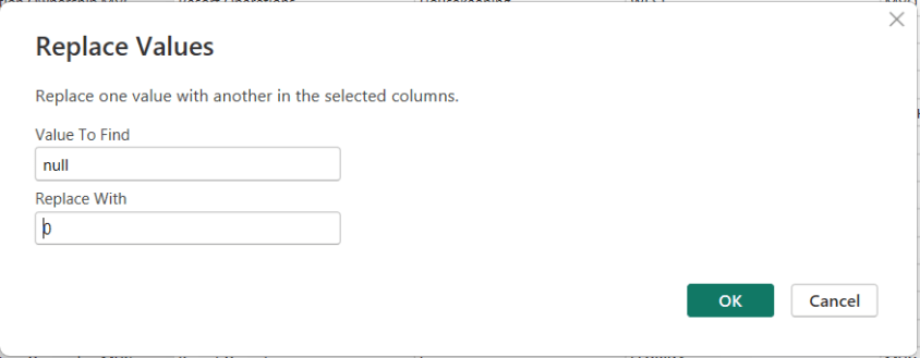
To replace NULLs, first select the column where the NULL values exist. Then choose Replace Values. When the dialog box appears, enter null as the value to find and replace, and specify the value you want to use instead—such as 0 for numeric columns or “Unknown” for text columns.

After confirming, Power Query automatically updates the column and records the step.

Thanks for reading!

Understanding the Power BI DAX “GENERATE / ROW” Pattern

The GENERATE / ROW pattern is an advanced but powerful DAX technique used to dynamically create rows and expand tables based on calculations. It is especially useful when you need to produce derived rows, combinations, or scenario-based expansions that don’t exist physically in your data model.

This article explains what the pattern is, when to use it, how it works, and provides practical examples. It assumes you are familiar with concepts such as row context, filter context, and iterators.


What Is the GENERATE / ROW Pattern?

At its core, the pattern combines two DAX functions:

  • GENERATE() – Iterates over a table and returns a union of tables generated for each row.
  • ROW() – Creates a single-row table with named columns and expressions.

Together, they allow you to:

  • Loop over an outer table
  • Generate one or more rows per input row
  • Shape those rows using calculated expressions

In effect, this pattern mimics a nested loop or table expansion operation.


Why This Pattern Exists

DAX does not support procedural loops like for or while.
Instead, iteration happens through table functions.

GENERATE() fills a critical gap by allowing you to:

  • Produce variable numbers of rows per input row
  • Apply row-level calculations while preserving relationships and context

Function Overview

GENERATE

GENERATE (
    table1,
    table2
)

  • table1: The outer table being iterated.
  • table2: A table expression evaluated for each row of table1.

The result is a flattened table containing all rows returned by table2 for every row in table1.


ROW

ROW (
    "ColumnName1", Expression1,
    "ColumnName2", Expression2
)

  • Returns a single-row table
  • Expressions are evaluated in the current row context

When Should You Use the GENERATE / ROW Pattern?

This pattern is ideal when:

✅ You Need to Create Derived Rows

Examples:

  • Generating “Start” and “End” rows per record
  • Creating multiple event types per transaction

✅ You Need Scenario or Category Expansion

Examples:

  • Actual vs Forecast vs Budget rows
  • Multiple pricing or discount scenarios

✅ You Need Row-Level Calculations That Produce Rows

Examples:

  • Expanding date ranges into multiple calculated milestones
  • Generating allocation rows per entity

❌ When Not to Use It

  • Simple aggregations → use SUMX, ADDCOLUMNS
  • Static lookup tables → use calculated tables or Power Query
  • High-volume fact tables without filtering (can be expensive)

Basic Example: Expanding Rows with Labels

Scenario

You have a Sales table:

OrderIDAmount
1100
2200

You want to generate two rows per order:

  • One for Gross
  • One for Net (90% of gross)

DAX Code

Sales Breakdown =
GENERATE (
    Sales,
    ROW (
        "Type", "Gross",
        "Value", Sales[Amount]
    )
    &
    ROW (
        "Type", "Net",
        "Value", Sales[Amount] * 0.9
    )
)


Result

OrderIDTypeValue
1Gross100
1Net90
2Gross200
2Net180

Key Concept: Context Transition

Inside ROW():

  • You are operating in row context
  • Columns from the outer table (Sales) are directly accessible
  • No need for EARLIER() or variables in most cases

This makes the pattern cleaner and easier to reason about.


Intermediate Example: Scenario Modeling

Scenario

You want to model multiple pricing scenarios for each product.

ProductBasePrice
A50
B100

Scenarios:

  • Standard (100%)
  • Discounted (90%)
  • Premium (110%)

DAX Code

Product Pricing Scenarios =
GENERATE (
    Products,
    UNION (
        ROW ( "Scenario", "Standard",   "Price", Products[BasePrice] ),
        ROW ( "Scenario", "Discounted", "Price", Products[BasePrice] * 0.9 ),
        ROW ( "Scenario", "Premium",    "Price", Products[BasePrice] * 1.1 )
    )
)


Result

ProductScenarioPrice
AStandard50
ADiscounted45
APremium55
BStandard100
BDiscounted90
BPremium110

Advanced Example: Date-Based Expansion

Scenario

For each project, generate two milestone rows:

  • Start Date
  • End Date
ProjectStartDateEndDate
X2024-01-012024-03-01

DAX Code

Project Milestones =
GENERATE (
    Projects,
    UNION (
        ROW (
            "Milestone", "Start",
            "Date", Projects[StartDate]
        ),
        ROW (
            "Milestone", "End",
            "Date", Projects[EndDate]
        )
    )
)

This is especially useful for timeline visuals or event-based reporting.


Performance Considerations ⚠️

The GENERATE / ROW pattern can be computationally expensive.

Best Practices

  • Filter the outer table as early as possible
  • Avoid using it on very large fact tables
  • Prefer calculated tables over measures when expanding rows
  • Test with realistic data volumes

Common Mistakes

❌ Using GENERATE When ADDCOLUMNS Is Enough

If you’re only adding columns—not rows—ADDCOLUMNS() is simpler and faster.

❌ Forgetting Table Shape Consistency

All ROW() expressions combined with UNION() must return the same column structure.

❌ Overusing It in Measures

This pattern is usually better suited for calculated tables, not measures.


Mental Model to Remember

Think of the GENERATE / ROW pattern as:

“For each row in this table, generate one or more calculated rows and stack them together.”

If that sentence describes your problem, this pattern is likely the right tool.


Final Thoughts

The GENERATE / ROW pattern is one of those DAX techniques that feels complex at first—but once understood, it unlocks entire classes of modeling and analytical solutions that are otherwise impossible.

Used thoughtfully, it can replace convoluted workarounds, reduce model complexity, and enable powerful scenario-based reporting.

Thanks for reading!

Exam Prep Hub for DP-600: Implementing Analytics Solutions Using Microsoft Fabric

This is your one-stop hub with information for preparing for the DP-600: Implementing Analytics Solutions Using Microsoft Fabric certification exam. Upon successful completion of the exam, you earn the Fabric Analytics Engineer Associate certification.

This hub provides information directly here, links to a number of external resources, tips for preparing for the exam, practice tests, and section questions to help you prepare. Bookmark this page and use it as a guide to ensure that you are fully covering all relevant topics for the exam and using as many of the resources available as possible. We hope you find it convenient and helpful.

Why do the DP-600: Implementing Analytics Solutions Using Microsoft Fabric exam to gain the Fabric Analytics Engineer Associate certification?

Most likely, you already know why you want to earn this certification, but in case you are seeking information on its benefits, here are a few:
(1) there is a possibility for career advancement because Microsoft Fabric is a leading data platform used by companies of all sizes, all over the world, and is likely to become even more popular
(2) greater job opportunities due to the edge provided by the certification
(3) higher earnings potential,
(4) you will expand your knowledge about the Fabric platform by going beyond what you would normally do on the job and
(5) it will provide immediate credibility about your knowledge, and
(6) it may, and it should, provide you with greater confidence about your knowledge and skills.


Important DP-600 resources:


DP-600: Skills measured as of October 31, 2025:

Here you can learn in a structured manner by going through the topics of the exam one-by-one to ensure full coverage; click on each hyperlinked topic below to go to more information about it:

Skills at a glance

  • Maintain a data analytics solution (25%-30%)
  • Prepare data (45%-50%)
  • Implement and manage semantic models (25%-30%)

Maintain a data analytics solution (25%-30%)

Implement security and governance

Maintain the analytics development lifecycle

Prepare data (45%-50%)

Get Data

Transform Data

Query and analyze data

Implement and manage semantic models (25%-30%)

Design and build semantic models

Optimize enterprise-scale semantic models


Practice Exams:

We have provided 2 practice exams with answers to help you prepare.

DP-600 Practice Exam 1 (60 questions with answer key)

DP-600 Practice Exam 2 (60 questions with answer key)


Good luck to you passing the DP-600: Implementing Analytics Solutions Using Microsoft Fabric certification exam and earning the Fabric Analytics Engineer Associate certification!

Implement Relationships, Such as Bridge Tables and Many-to-Many Relationships

This post is a part of the DP-600: Implementing Analytics Solutions Using Microsoft Fabric Exam Prep Hub; and this topic falls under these sections: 
Implement and manage semantic models (25-30%)
--> Design and build semantic models
--> Implement Relationships, Such as Bridge Tables

and Many-to-Many Relationships

Why Relationships Matter in Semantic Models

In Microsoft Fabric and Power BI semantic models, relationships define how tables interact and how filters propagate across data. Well-designed relationships are critical for:

  • Accurate aggregations
  • Predictable filtering behavior
  • Correct DAX calculations
  • Optimal query performance

While one-to-many relationships are preferred, real-world data often requires handling many-to-many relationships using techniques such as bridge tables.


Common Relationship Types in Semantic Models

1. One-to-Many (Preferred)

  • One dimension row relates to many fact rows
  • Most common and performant relationship
  • Typical in star schemas

Example:

  • DimCustomer → FactSales

2. Many-to-Many

  • Multiple rows in one table relate to multiple rows in another
  • More complex filtering behavior
  • Can negatively impact performance if not modeled correctly

Example:

  • Customers associated with multiple regions
  • Products assigned to multiple categories

Understanding Many-to-Many Relationships

Native Many-to-Many Relationships

Power BI supports direct many-to-many relationships, but these should be used carefully.

Characteristics:

  • Cardinality: Many-to-many
  • Filters propagate ambiguously
  • DAX becomes harder to reason about

Exam Tip:
Direct many-to-many relationships are supported but not always recommended for complex models.


Bridge Tables (Best Practice)

A bridge table (also called a factless fact table) resolves many-to-many relationships by introducing an intermediate table.

What Is a Bridge Table?

A table that:

  • Contains keys from two related entities
  • Has no numeric measures
  • Enables controlled filtering paths

Example Scenario

Business case:
Products can belong to multiple categories.

Tables:

  • DimProduct (ProductID, Name)
  • DimCategory (CategoryID, CategoryName)
  • BridgeProductCategory (ProductID, CategoryID)

Relationships:

  • DimProduct → BridgeProductCategory (one-to-many)
  • DimCategory → BridgeProductCategory (one-to-many)

This converts a many-to-many relationship into two one-to-many relationships.


Benefits of Using Bridge Tables

BenefitDescription
Predictable filteringClear filter paths
Better DAX controlEasier to write and debug measures
Improved performanceAvoids ambiguous joins
ScalabilityHandles complex relationships cleanly

Filter Direction Considerations

Single vs Bidirectional Filters

  • Single direction (recommended):
    Filters flow from dimension → bridge → fact
  • Bidirectional:
    Can simplify some scenarios but increases ambiguity

Exam Guidance:

  • Use single-direction filters by default
  • Enable bidirectional filtering only when required and understood

Many-to-Many and DAX Implications

When working with many-to-many relationships:

  • Measures may return unexpected results
  • DISTINCTCOUNT is commonly required
  • Explicit filtering using DAX functions may be necessary

Common DAX patterns:

  • CALCULATE
  • TREATAS
  • CROSSFILTER (advanced)

Relationship Best Practices for DP-600

  • Favor star schemas with one-to-many relationships
  • Use bridge tables instead of direct many-to-many when possible
  • Avoid unnecessary bidirectional filters
  • Validate relationship cardinality and direction
  • Test measures under different filtering scenarios

Common Exam Scenarios

You may see questions like:

  • “How do you model a relationship where products belong to multiple categories?”
  • “What is the purpose of a bridge table?”
  • “What are the risks of many-to-many relationships?”

Correct answers typically emphasize:

  • Bridge tables
  • Controlled filter propagation
  • Avoiding ambiguous relationships

Star Schema vs Many-to-Many Models

FeatureStar SchemaMany-to-Many
ComplexityLowHigher
PerformanceBetterLower
DAX simplicityHighLower
Use casesMost analyticsSpecialized scenarios

Summary

Implementing relationships correctly is foundational to building reliable semantic models in Microsoft Fabric:

  • One-to-many relationships are preferred
  • Many-to-many relationships should be handled carefully
  • Bridge tables provide a scalable, exam-recommended solution
  • Clear relationships lead to accurate analytics and simpler DAX

Exam Tip

If a question involves multiple entities relating to each other, or many-to-many relationships, the most likely answer usually includes using a “bridge table”.

Practice Questions:

Here are 10 questions to test and help solidify your learning and knowledge. As you review these and other questions in your preparation, make sure to …

  • Identifying and understand why an option is correct (or incorrect) — not just which one
  • Look for and understand the usage scenario of keywords in exam questions to guide you
  • Expect scenario-based questions rather than direct definitions

1. Which relationship type is generally preferred in Power BI semantic models?

A. Many-to-many
B. One-to-one
C. One-to-many
D. Bidirectional many-to-many

Correct Answer: C

Explanation:
One-to-many relationships provide predictable filter propagation, better performance, and simpler DAX calculations.


2. What is the primary purpose of a bridge table?

A. Store aggregated metrics
B. Normalize dimension attributes
C. Resolve many-to-many relationships
D. Improve data refresh performance

Correct Answer: C

Explanation:
Bridge tables convert many-to-many relationships into two one-to-many relationships, improving model clarity and control.


3. Which characteristic best describes a bridge table?

A. Contains numeric measures
B. Stores transactional data
C. Contains keys from related tables only
D. Is always filtered bidirectionally

Correct Answer: C

Explanation:
Bridge tables typically contain only keys (foreign keys) and no measures, enabling relationship resolution.


4. What is a common risk of using native many-to-many relationships directly?

A. They cannot be refreshed
B. They cause data duplication
C. They create ambiguous filter propagation
D. They are unsupported in Fabric

Correct Answer: C

Explanation:
Native many-to-many relationships can result in ambiguous filtering and unpredictable aggregation results.


5. In a bridge table scenario, how are relationships typically defined?

A. Many-to-many on both sides
B. One-to-one from both dimensions
C. One-to-many from each dimension to the bridge
D. Bidirectional many-to-one

Correct Answer: C

Explanation:
Each dimension connects to the bridge table using a one-to-many relationship.


6. When should bidirectional filtering be enabled?

A. Always, for simplicity
B. Only when necessary and well-understood
C. Only on fact tables
D. Never in semantic models

Correct Answer: B

Explanation:
Bidirectional filters can be useful but introduce complexity and ambiguity if misused.


7. Which scenario is best handled using a bridge table?

A. A customer has one address
B. A sale belongs to one product
C. A product belongs to multiple categories
D. A date table relates to a fact table

Correct Answer: C

Explanation:
Products belonging to multiple categories is a classic many-to-many scenario requiring a bridge table.


8. How does a properly designed bridge table affect DAX measures?

A. Makes measures harder to write
B. Requires custom SQL logic
C. Enables predictable filter behavior
D. Eliminates the need for CALCULATE

Correct Answer: C

Explanation:
Bridge tables create clear filter paths, making DAX behavior more predictable and reliable.


9. Which DAX function is commonly used to handle complex many-to-many filtering scenarios?

A. SUMX
B. RELATED
C. TREATAS
D. LOOKUPVALUE

Correct Answer: C

Explanation:
TREATAS is often used to apply filters across tables that are not directly related.


10. For DP-600 exam questions involving many-to-many relationships, which solution is typically preferred?

A. Direct many-to-many relationships
B. Denormalized fact tables
C. Bridge tables with one-to-many relationships
D. Duplicate dimension tables

Correct Answer: C

Explanation:
The exam emphasizes scalable, maintainable modeling practices — bridge tables are the recommended solution.


Select, Filter, and Aggregate Data Using DAX

This post is a part of the DP-600: Implementing Analytics Solutions Using Microsoft Fabric Exam Prep Hub; and this topic falls under these sections: 
Prepare data
--> Query and analyze data
--> Select, Filter, and Aggregate Data Using DAX

Data Analysis Expressions (DAX) is a formula language used to create dynamic calculations in Power BI semantic models. Unlike SQL or KQL, DAX works within the analytical model and is designed for filter context–aware calculations, interactive reporting, and business logic. For DP-600, you should understand how to use DAX to select, filter, and aggregate data within a semantic model for analytics and reporting.


What Is DAX?

DAX is similar to Excel formulas but optimized for relational, in-memory analytics. It is used in:

  • Measures (dynamic calculations)
  • Calculated columns (row-level derived values)
  • Calculated tables (additional, reusable query results)

In a semantic model, DAX queries run in response to visuals and can produce results based on current filters and slicers.


Selecting Data in DAX

DAX itself doesn’t use a traditional SELECT statement like SQL. Instead:

  • Data is selected implicitly by filter context
  • DAX measures operate over table columns referenced in expressions

Example of a simple DAX measure selecting and displaying sales:

Total Sales = SUM(Sales[SalesAmount])

Here:

  • Sales[SalesAmount] references the column in the Sales table
  • The measure returns the sum of all values in that column

Filtering Data in DAX

Filtering in DAX is context-driven and can be applied in multiple ways:

1. Implicit Filters

Visual-level filters and slicers automatically apply filters to DAX measures.

Example:
A card visual showing Total Sales will reflect only the filtered subset by product or date.

2. FILTER Function

Used within measures or calculated tables to narrow down rows:

HighValueSales = CALCULATE(
    SUM(Sales[SalesAmount]),
    FILTER(Sales, Sales[SalesAmount] > 1000)
)

Here:

  • FILTER returns a table with rows meeting the condition
  • CALCULATE modifies the filter context

3. CALCULATE as Filter Modifier

CALCULATE changes the context under which a measure evaluates:

SalesLastYear = CALCULATE(
    [Total Sales],
    SAMEPERIODLASTYEAR(Date[Date])
)

This measure selects data for the previous year based on current filters.


Aggregating Data in DAX

Aggregation in DAX is done using built-in functions and is influenced by filter context.

Common Aggregation Functions

  • SUM() — totals a numeric column
  • AVERAGE() — computes the mean
  • COUNT() / COUNTA() — row counts
  • MAX() / MIN() — extreme values
  • SUMX() — row-by-row iteration and sum

Example of row-by-row aggregation:

Total Profit = SUMX(
    Sales,
    Sales[SalesAmount] - Sales[Cost]
)

This computes the difference per row and then sums it.


Filter Context and Row Context

Understanding how DAX handles filter context and row context is essential:

  • Filter context: Set by the report (slicers, column filters) or modified by CALCULATE
  • Row context: Used in calculated columns and iteration functions (SUMX, FILTER)

DAX measures always respect the current filter context unless explicitly modified.


Grouping and Summarization

While DAX doesn’t use GROUP BY in the same way SQL does, measures inherently aggregate over groups determined by filter context or visual grouping.

Example:
In a table visual grouped by Product Category, the measure Total Sales returns aggregated values per category automatically.


Time Intelligence Functions

DAX includes built-in functions for time-based aggregation:

  • TOTALYTD(), TOTALQTD(), TOTALMTD() — year-to-date, quarter-to-date, month-to-date
  • SAMEPERIODLASTYEAR() — compare values year-over-year
  • DATESINPERIOD() — custom period

Example:

SalesYTD = TOTALYTD(
    [Total Sales],
    Date[Date]
)


Best Practices

  • Use measures, not calculated columns, for dynamic, filter-sensitive aggregations.
  • Let visuals control filter context via slicers, rows, and columns.
  • Avoid unnecessary row-by-row calculations when simple aggregation functions suffice.
  • Explicitly use CALCULATE to modify filter context for advanced scenarios.

When to Use DAX vs SQL/KQL

ScenarioBest Tool
Static relational queryingSQL
Streaming/event analyticsKQL
Report-level dynamic calculationsDAX
Interactive dashboards with slicersDAX

Example Use Cases

1. Total Sales Measure

Total Sales = SUM(Sales[SalesAmount])

2. Filtered Sales for Big Orders

Big Orders Sales = CALCULATE(
    [Total Sales],
    Sales[SalesAmount] > 1000
)

3. Year-over-Year Sales

Sales YOY = CALCULATE(
    [Total Sales],
    SAMEPERIODLASTYEAR(Date[Date])
)


Key Takeaways for the Exam

  • DAX operates based on filter context and evaluates measures dynamically.
  • There is no explicit SELECT statement — rather, measures compute values based on current context.
  • Use CALCULATE to change filter context.
  • Aggregation functions (e.g., SUM, COUNT, AVERAGE) are fundamental to summarizing data.
  • Filtering functions like FILTER and time intelligence functions enhance analytical flexibility.

Final Exam Tips

  • If a question mentions interactive reports, dynamic filters, slicers, or time-based comparisons, DAX is likely the right language to use for the solution.
  • Measures + CALCULATE + filter context appear frequently.
  • If the question mentions slicers, visuals, or dynamic results, think DAX measure.
  • Time intelligence functions are high-value topics.

Practice Questions:

Here are 10 questions to test and help solidify your learning and knowledge. As you review these and other questions in your preparation, make sure to …

  • Identifying and understand why an option is correct (or incorrect) — not just which one
  • Look for and understand the usage scenario of keywords in exam questions to guide you
  • Expect scenario-based questions rather than direct definitions

1. Which DAX function is primarily used to modify the filter context of a calculation?

A. FILTER
B. SUMX
C. CALCULATE
D. ALL

Correct answer: ✅ C
Explanation: CALCULATE changes the filter context under which an expression is evaluated.


2. A Power BI report contains slicers for Year and Product. A measure returns different results as slicers change. What concept explains this behavior?

A. Row context
B. Filter context
C. Evaluation context
D. Query context

Correct answer: ✅ B
Explanation: Filter context is affected by slicers, filters, and visual interactions.


3. Which DAX function iterates row by row over a table to perform a calculation?

A. SUM
B. COUNT
C. AVERAGE
D. SUMX

Correct answer: ✅ D
Explanation: SUMX evaluates an expression for each row and then aggregates the results.


4. You want to calculate total sales only for transactions greater than $1,000. Which approach is correct?

A.

SUM(Sales[SalesAmount] > 1000)

B.

FILTER(Sales, Sales[SalesAmount] > 1000)

C.

CALCULATE(
    SUM(Sales[SalesAmount]),
    Sales[SalesAmount] > 1000
)

D.

SUMX(Sales, Sales[SalesAmount] > 1000)

Correct answer: ✅ C
Explanation: CALCULATE applies a filter condition while aggregating.


5. Which DAX object is evaluated dynamically based on report filters and slicers?

A. Calculated column
B. Calculated table
C. Measure
D. Relationship

Correct answer: ✅ C
Explanation: Measures respond dynamically to filter context; calculated columns do not.


6. Which function is commonly used to calculate year-to-date (YTD) values in DAX?

A. DATESINPERIOD
B. SAMEPERIODLASTYEAR
C. TOTALYTD
D. CALCULATE

Correct answer: ✅ C
Explanation: TOTALYTD is designed for year-to-date aggregations.


7. A DAX measure returns different totals when placed in a table visual grouped by Category. Why does this happen?

A. The measure contains row context
B. The table visual creates filter context
C. The measure is recalculated per row
D. Relationships are ignored

Correct answer: ✅ B
Explanation: Visual grouping applies filter context automatically.


8. Which DAX function returns a table instead of a scalar value?

A. SUM
B. AVERAGE
C. FILTER
D. COUNT

Correct answer: ✅ C
Explanation: FILTER returns a table that can be consumed by other functions like CALCULATE.


9. Which scenario is the best use case for DAX instead of SQL or KQL?

A. Cleaning raw data before ingestion
B. Transforming streaming event data
C. Creating interactive report-level calculations
D. Querying flat files in a lakehouse

Correct answer: ✅ C
Explanation: DAX excels at dynamic, interactive calculations in semantic models.


10. What is the primary purpose of the SAMEPERIODLASTYEAR function?

A. Aggregate values by fiscal year
B. Remove filters from a date column
C. Compare values to the previous year
D. Calculate rolling averages

Correct answer: ✅ C
Explanation: It shifts the date context back one year for year-over-year analysis.


Select, Filter, and Aggregate Data Using SQL

This post is a part of the DP-600: Implementing Analytics Solutions Using Microsoft Fabric Exam Prep Hub; and this topic falls under these sections: 
Prepare data
--> Query and analyze data
--> Select, Filter, and Aggregate Data Using SQL

Working with SQL to select, filter, and aggregate data is a core skill for analytics engineers using Microsoft Fabric. Whether querying data in a warehouse, lakehouse SQL analytics endpoint, or semantic model via DirectQuery, SQL enables precise data retrieval and summarization for reporting, dashboards, and analytics solutions.

For DP-600, you should understand how to construct SQL queries that perform:

  • Selecting specific data columns
  • Filtering rows based on conditions
  • Aggregating values with grouping and summary functions

SQL Data Selection

Selecting data refers to using the SELECT clause to choose which columns or expressions to return.

Example:

SELECT
    CustomerID,
    OrderDate,
    SalesAmount
FROM Sales;

  • Use * to return all columns:
    SELECT * FROM Sales;
  • Use expressions to compute derived values: SELECT OrderDate, SalesAmount, SalesAmount * 1.1 AS AdjustedRevenue FROM Sales;

Exam Tip: Be purposeful in selecting only needed columns to improve performance.


SQL Data Filtering

Filtering data determines which rows are returned based on conditions using the WHERE clause.

Basic Filtering:

SELECT *
FROM Sales
WHERE OrderDate >= '2025-01-01';

Combined Conditions:

  • AND: WHERE Country = 'USA' AND SalesAmount > 1000
  • OR: WHERE Region = 'East' OR Region = 'West'

Null and Missing Value Filters:

WHERE SalesAmount IS NOT NULL

Exam Tip: Understand how WHERE filters reduce dataset size before aggregation.


SQL Aggregation

Aggregation summarizes grouped rows using functions like SUM, COUNT, AVG, MIN, and MAX.

Basic Aggregation:

SELECT
    SUM(SalesAmount) AS TotalSales
FROM Sales;

Grouped Aggregation:

SELECT
    Country,
    SUM(SalesAmount) AS TotalSales,
    COUNT(*) AS OrderCount
FROM Sales
GROUP BY Country;

Filtering After Aggregation:

Use HAVING instead of WHERE to filter aggregated results:

SELECT
    Country,
    SUM(SalesAmount) AS TotalSales
FROM Sales
GROUP BY Country
HAVING SUM(SalesAmount) > 100000;

Exam Tip:

  • Use WHERE for row-level filters before grouping.
  • Use HAVING to filter group-level aggregates.

Combining Select, Filter, and Aggregate

A complete SQL query often blends all three:

SELECT
    ProductCategory,
    COUNT(*) AS Orders,
    SUM(SalesAmount) AS TotalSales,
    AVG(SalesAmount) AS AvgSale
FROM Sales
WHERE OrderDate BETWEEN '2025-01-01' AND '2025-12-31'
GROUP BY ProductCategory
ORDER BY TotalSales DESC;

This example:

  • Selects specific columns and expressions
  • Filters by date range
  • Aggregates by product category
  • Orders results by summary metric

SQL in Different Fabric Workloads

WorkloadSQL Usage
WarehouseStandard T-SQL for BI queries
Lakehouse SQL AnalyticsSQL against Delta tables
Semantic Models via DirectQuerySQL pushed to source where supported
Dataflows/Power QuerySQL-like operations through M (not direct SQL)

Performance and Pushdown

When using SQL in Fabric:

  • Engines push filters and aggregations down to the data source for performance.
  • Select only needed columns early to limit data movement.
  • Avoid SELECT * in production queries unless necessary.

Key SQL Concepts for the Exam

ConceptWhy It Matters
SELECTDefines what data to retrieve
WHEREFilters data before aggregation
GROUP BYOrganizes rows into groups
HAVINGFilters after aggregation
Aggregate functionsSummarize numeric data

Understanding how these work together is essential for creating analytics-ready datasets.


Common Exam Scenarios

You may be asked to:

  • Write SQL to filter data based on conditions
  • Summarize data across groups
  • Decide whether to use WHERE or HAVING
  • Identify the correct SQL pattern for a reporting requirement

Example exam prompt:

“Which SQL query correctly returns the total sales per region, only for regions with more than 1,000 orders?”

Understanding aggregate filters (HAVING) and groupings will be key.


Final Exam Tips

If a question mentions:

  • “Return summary metrics”
  • “Only include rows that meet conditions”
  • “Group results by category”

…you’re looking at combining SELECT, WHERE, and GROUP BY in SQL.

  • WHERE filters rows before aggregation
  • HAVING filters after aggregation
  • GROUP BY is required for per-group metrics
  • Use aggregate functions intentionally
  • Performance matters — avoid unnecessary columns

Practice Questions:

Here are 10 questions to test and help solidify your learning and knowledge. As you review these and other questions in your preparation, make sure to …

  • Identifying and understand why an option is correct (or incorrect) — not just which one
  • Look for and understand the usage scenario of keywords in exam questions to guide you
  • Expect scenario-based questions rather than direct definitions

1. Which SQL clause is used to filter rows before aggregation occurs?

A. HAVING
B. GROUP BY
C. WHERE
D. ORDER BY

Correct Answer: C

Explanation:
The WHERE clause filters individual rows before any aggregation or grouping takes place. HAVING filters results after aggregation.


2. You need to calculate total sales per product category. Which clause is required?

A. WHERE
B. GROUP BY
C. ORDER BY
D. HAVING

Correct Answer: B

Explanation:
GROUP BY groups rows so aggregate functions (such as SUM) can be calculated per category.


3. Which function returns the number of rows in each group?

A. SUM()
B. COUNT()
C. AVG()
D. MAX()

Correct Answer: B

Explanation:
COUNT() counts the number of rows in a group. It is commonly used to count records or transactions.


4. Which query correctly filters aggregated results?

A.

WHERE SUM(SalesAmount) > 10000

B.

HAVING SUM(SalesAmount) > 10000

C.

GROUP BY SUM(SalesAmount) > 10000

D.

ORDER BY SUM(SalesAmount) > 10000

Correct Answer: B

Explanation:
HAVING is used to filter aggregated values. WHERE cannot reference aggregate functions.


5. Which SQL statement returns the total number of orders?

A.

SELECT COUNT(*) FROM Orders;

B.

SELECT SUM(*) FROM Orders;

C.

SELECT TOTAL(Orders) FROM Orders;

D.

SELECT COUNT(Orders) FROM Orders;

Correct Answer: A

Explanation:
COUNT(*) counts all rows in a table, making it the correct way to return total order count.


6. Which clause is used to sort aggregated query results?

A. GROUP BY
B. WHERE
C. ORDER BY
D. HAVING

Correct Answer: C

Explanation:
ORDER BY sorts the final result set, including aggregated columns.


7. What happens if a column in the SELECT statement is not included in the GROUP BY clause or an aggregate function?

A. The query runs but returns incorrect results
B. SQL automatically groups it
C. The query fails
D. The column is ignored

Correct Answer: C

Explanation:
In SQL, any column in SELECT must either be aggregated or included in GROUP BY.


8. Which query returns average sales amount per country?

A.

SELECT Country, AVG(SalesAmount)
FROM Sales;

B.

SELECT Country, AVG(SalesAmount)
FROM Sales
GROUP BY Country;

C.

SELECT Country, SUM(SalesAmount)
GROUP BY Country;

D.

SELECT AVG(SalesAmount)
FROM Sales
GROUP BY Country;

Correct Answer: B

Explanation:
Grouping by Country allows AVG(SalesAmount) to be calculated per country.


9. Which filter removes rows with NULL values in a column?

A.

WHERE SalesAmount = NULL

B.

WHERE SalesAmount <> NULL

C.

WHERE SalesAmount IS NOT NULL

D.

WHERE NOT NULL SalesAmount

Correct Answer: C

Explanation:
SQL uses IS NULL and IS NOT NULL to check for null values.


10. Which SQL pattern is most efficient for analytics queries in Microsoft Fabric?

A. Selecting all columns and filtering later
B. Using SELECT * for simplicity
C. Filtering early and selecting only needed columns
D. Aggregating without grouping

Correct Answer: C

Explanation:
Filtering early and selecting only required columns improves performance by reducing data movement—an important Fabric best practice.


Select, Filter, and Aggregate Data by Using the Visual Query Editor

This post is a part of the DP-600: Implementing Analytics Solutions Using Microsoft Fabric Exam Prep Hub; and this topic falls under these sections: 
Prepare data
--> Query and analyze data
--> Select, Filter, and Aggregate Data by Using the Visual Query Editor

In Microsoft Fabric, the Visual Query Editor (VQE) provides a low-code, graphical experience for querying data across lakehouses, warehouses, and semantic models. It allows analytics engineers to explore, shape, and summarize data without writing SQL or KQL, while still generating optimized queries behind the scenes.

For the DP-600 exam, you should understand what the Visual Query Editor is, where it’s used, and how to perform common data analysis tasks such as selecting columns, filtering rows, and aggregating data.


What Is the Visual Query Editor?

The Visual Query Editor is a graphical query-building interface available in multiple Fabric experiences, including:

  • Lakehouse SQL analytics endpoint
  • Warehouse
  • Power BI (Direct Lake and DirectQuery scenarios)
  • Data exploration within Fabric items

Instead of writing queries manually, you interact with:

  • Tables and columns
  • Drag-and-drop operations
  • Menus for filters, grouping, and aggregations

Fabric then translates these actions into optimized SQL or engine-specific queries.


Selecting Data

Selecting data in the Visual Query Editor focuses on choosing the right columns and datasets for analysis.

Key Capabilities

  • Select or deselect columns from one or more tables
  • Rename columns for readability
  • Reorder columns for analysis or reporting
  • Combine columns from related tables (via existing relationships)

Exam Tips

  • Selecting fewer columns improves performance and reduces data transfer.
  • Column renaming in VQE affects the query result, not the underlying table schema.
  • The Visual Query Editor respects relationships defined in semantic models and warehouses.

Filtering Data

Filtering allows you to limit rows based on conditions, ensuring only relevant data is included.

Common Filter Types

  • Equality filters (e.g., Status = "Active")
  • Range filters (e.g., dates, numeric thresholds)
  • Text filters (contains, starts with, ends with)
  • Null / non-null filters
  • Relative date filters (last 7 days, current month)

Where Filtering Is Applied

  • At the query level, not permanently in the data source
  • Before aggregation (important for correct results)

Exam Tips

  • Filters applied in the Visual Query Editor are executed at the data source when possible (query folding).
  • Filtering early improves performance and reduces memory usage.
  • Be aware of how filters interact with aggregations.

Aggregating Data

Aggregation summarizes data by grouping rows and applying calculations.

Common Aggregations

  • Sum
  • Count / Count Distinct
  • Average
  • Min / Max

Grouping Data

  • Select one or more columns as group-by fields
  • Apply aggregations to numeric or date columns
  • Results return one row per group

Examples

  • Total sales by product category
  • Count of orders per customer
  • Average response time by day

Exam Tips

  • Aggregations in the Visual Query Editor are conceptually similar to GROUP BY in SQL.
  • Aggregated queries reduce dataset size and improve performance.
  • Understand the difference between row-level data and aggregated results.

Behind the Scenes: Generated Queries

Although the Visual Query Editor is low-code, Fabric generates:

  • SQL queries for warehouses and lakehouse SQL endpoints
  • Optimized engine-specific queries for semantic models

This ensures:

  • Efficient execution
  • Compatibility with Direct Lake and DirectQuery
  • Consistent results across Fabric experiences

Exam Tip

You are not required to read or write the generated SQL, but you should understand that the Visual Query Editor does not bypass query optimization.


When to Use the Visual Query Editor

Use the Visual Query Editor when:

  • Quickly exploring unfamiliar datasets
  • Building queries without writing code
  • Creating reusable query logic for reports
  • Teaching or collaborating with less SQL-focused users

Avoid it when:

  • Complex transformations are required (use SQL, Spark, or Dataflows)
  • Highly customized logic is needed beyond supported operations

Key Exam Takeaways

For the DP-600 exam, remember:

  • The Visual Query Editor is a graphical query-building tool in Microsoft Fabric.
  • It supports selecting columns, filtering rows, and aggregating data.
  • Operations are translated into optimized queries executed at the data source.
  • Filtering occurs before aggregation, affecting results and performance.
  • It is commonly used with lakehouses, warehouses, and semantic models.

Practice Questions:

Here are 10 questions to test and help solidify your learning and knowledge. As you review these and other questions in your preparation, make sure to …

  • Identifying and understand why an option is correct (or incorrect) — not just which one
  • Look for and understand the usage scenario of keywords in exam questions to guide you
  • Expect scenario-based questions rather than direct definitions
  • Know the purpose and scope of the Visual Query Editor
  • Know how to selecting, filtering, and aggregating data
  • Understand execution order and performance implications
  • Know when to use (and not use) the Visual Query Editor

Question 1

What is the primary purpose of the Visual Query Editor in Microsoft Fabric?

A. To permanently modify table schemas
B. To build queries visually without writing SQL
C. To replace semantic models
D. To manage workspace permissions

Correct Answer: B

Explanation:
The Visual Query Editor provides a low-code, graphical interface for building queries. It does not modify schemas, replace models, or manage security.


Question 2

When you deselect a column in the Visual Query Editor, what happens?

A. The column is deleted from the source table
B. The column is hidden permanently for all users
C. The column is excluded only from the query results
D. The column data type is changed

Correct Answer: C

Explanation:
Column selection affects only the query output, not the underlying data or schema.


Question 3

Why is it considered a best practice to select only required columns in a query?

A. It enforces data security
B. It reduces query complexity and improves performance
C. It enables Direct Lake mode
D. It prevents duplicate rows

Correct Answer: B

Explanation:
Selecting fewer columns reduces data movement and memory usage, leading to better performance.


Question 4

Which type of filter is commonly used to restrict data to a recent time period?

A. Equality filter
B. Text filter
C. Relative date filter
D. Aggregate filter

Correct Answer: C

Explanation:
Relative date filters (e.g., “Last 30 days”) dynamically adjust based on the current date and are commonly used in analytics.


Question 5

At what stage of query execution are filters applied in the Visual Query Editor?

A. After aggregation
B. After the query result is returned
C. Before aggregation
D. Only in the Power BI report layer

Correct Answer: C

Explanation:
Filters are applied before aggregation, ensuring accurate summary results and better performance.


Question 6

Which aggregation requires grouping to produce meaningful results?

A. SUM
B. COUNT
C. GROUP BY
D. MIN

Correct Answer: C

Explanation:
Grouping defines how rows are summarized. Aggregations like SUM or COUNT rely on GROUP BY logic to produce per-group results.


Question 7

You want to see total sales by product category. Which Visual Query Editor actions are required?

A. Filter Product Category and sort by Sales
B. Group by Product Category and apply SUM to Sales
C. Count Product Category and filter Sales
D. Rename Product Category and aggregate rows

Correct Answer: B

Explanation:
This scenario requires grouping on Product Category and applying a SUM aggregation to the Sales column.


Question 8

What happens behind the scenes when you build a query using the Visual Query Editor?

A. Fabric stores a cached dataset only
B. Fabric generates optimized SQL or engine-specific queries
C. Fabric converts the query into DAX
D. Fabric disables query folding

Correct Answer: B

Explanation:
The Visual Query Editor translates visual actions into optimized queries (such as SQL) that execute at the data source.


Question 9

Which Fabric items commonly support querying through the Visual Query Editor?

A. Pipelines and notebooks only
B. Dashboards only
C. Lakehouses, warehouses, and semantic models
D. Eventhouses only

Correct Answer: C

Explanation:
The Visual Query Editor is widely used across lakehouses, warehouses, and semantic models in Fabric.


Question 10

When should you avoid using the Visual Query Editor?

A. When exploring new datasets
B. When building quick aggregations
C. When complex transformation logic is required
D. When filtering data

Correct Answer: C

Explanation:
For advanced or complex transformations, SQL, Spark, or Dataflows are more appropriate than the Visual Query Editor.


Filter Data

This post is a part of the DP-600: Implementing Analytics Solutions Using Microsoft Fabric Exam Prep Hub; and this topic falls under these sections: 
Prepare data
--> Transform data
--> Filter data

Filtering data is one of the most fundamental transformation operations used when preparing analytics data. It ensures that only relevant, valid, and accurate records are included in curated tables or models. Filtering improves performance, reduces unnecessary processing overhead, and helps enforce business logic early in the analytics pipeline.

In Microsoft Fabric, filtering occurs at multiple transformation layers — from ingestion tools to interactive modeling. For the DP-600 exam, you should understand where, why, and how to filter data effectively using various tools and technologies within Fabric.


Why Filter Data?

Filtering data serves several key purposes in analytics:

1. Improve Query and Report Performance

  • Reduces the amount of data scanned and processed
  • Enables faster refresh and retrieval

2. Enforce Business Logic

  • Excludes irrelevant segments (e.g., test data, canceled transactions)
  • Supports clean analytical results

3. Prepare Analytics-Ready Data

  • Limits datasets to required time periods or categories
  • Produces smaller, focused outputs for reporting

4. Reduce Cost

  • Smaller processing needs reduce compute and storage overhead

Where Filtering Happens in Microsoft Fabric

Filtering can be implemented at multiple stages:

LayerHow You Filter
Power Query (Dataflows Gen2 / Lakehouse)UI filters or M code
SQL (Warehouse & Lakehouse SQL analytics)WHERE clauses
Spark (Lakehouse Notebooks)DataFrame filter() / where()
Pipelines (Data Movement)Source filters or query-based extraction
Semantic Models (Power BI / DAX)Query filters, slicers, and row-level security

Filtering early, as close to the data source as possible, ensures better performance downstream.


Tools and Techniques

1. Power Query (Low-Code)

Power Query provides a user-friendly interface to filter rows:

  • Text filters: Equals, Begins With, Contains, etc.
  • Number filters: Greater than, Between, Top N, etc.
  • Date filters: Before, After, This Month, Last 12 Months, etc.
  • Remove blank or null values

These filters are recorded as transformation steps and can be reused or versioned.


2. SQL (Warehouses & Lakehouses)

SQL filtering uses the WHERE clause:

SELECT *
FROM Sales
WHERE OrderDate >= '2025-01-01'
  AND Country = 'USA';

SQL filtering is efficient and pushed down to the engine, reducing row counts early.


3. Spark (Notebooks)

Filtering in Spark (PySpark example):

filtered_df = df.filter(df["SalesAmount"] > 1000)

Or with SQL in Spark:

SELECT *
FROM sales
WHERE SalesAmount > 1000;

Spark filtering is optimized for distributed processing across big datasets.


4. Pipelines (Data Movement)

During ingestion or ETL, you can apply filters in:

  • Copy activity query filters
  • Source queries
  • Pre-processing steps

This ensures only needed rows land in the target store.


5. Semantic Model Filters

In Power BI and semantic models, filtering can happen as:

  • Report filters
  • Slicers and visuals
  • Row-Level Security (RLS) — security-driven filtering

These filters control what users see rather than what data is stored.


Business and Data Quality Scenarios

Filtering is often tied to business needs such as:

  • Excluding invalid, test, or archived records
  • Restricting to active customers only
  • Selecting a specific date range (e.g., last fiscal year)
  • Filtering data for regional or product segments

Filtering vs Security

It’s important to distinguish filtering for transformation from security filters:

FilteringSecurity
Removes unwanted rows during transformationControls what users are allowed to see
Improves performanceEnforces access control
Happens before modelingHappens during query evaluation

Best Practices

When filtering data in Microsoft Fabric:

  • Filter early in the pipeline to reduce volume
  • Use pushdown filters in SQL when querying large sources
  • Document filtering logic for audit and governance
  • Combine filters logically (AND/OR) to match business rules
  • Avoid filtering in the semantic model when it can be done upstream

Common Exam Scenarios

You may be asked to:

  • Choose the correct tool and stage for filtering
  • Translate business rules into filter logic
  • Recognize when filtering improves performance
  • Identify risks of filtering too late or in the wrong layer

Example exam prompt:
A dataset should exclude test transactions and include only the last 12 months of sales. Which transformation step should be applied and where?
The correct answer will involve filtering early with SQL or Power Query before modeling.


Key Takeaways

  • Filtering data is a core part of preparing analytics-ready datasets.
  • Multiple Fabric components support filtering (Power Query, SQL, Spark, pipelines).
  • Filtering early improves performance and reduces unnecessary workload.
  • Understand filtering in context — transformation vs. security.

Final Exam Tips

  • When a question asks about reducing dataset size, improving performance, or enforcing business logic before loading into a model, filtering is often the correct action — and it usually belongs upstream.
  • Filter early and upstream whenever possible
  • Use SQL or Power Query for transformation-level filtering
  • Avoid relying solely on report-level filters for large datasets
  • Distinguish filtering for performance from security filtering

Practice Questions:

Here are 10 questions to test and help solidify your learning and knowledge. As you review these and other questions in your preparation, make sure to …

  • Identifying and understand why an option is correct (or incorrect) — not just which one
  • Look for and understand the usage scenario of keywords in exam questions to guide you
  • Expect scenario-based questions rather than direct definitions

Question 1

What is the primary purpose of filtering data during the transformation phase?

A. To enforce user-level security
B. To reduce data volume and improve performance
C. To encrypt sensitive columns
D. To normalize data structures

Correct Answer: B

Explanation:
Filtering removes unnecessary rows early in the pipeline, reducing data volume, improving performance, and lowering compute costs. Security and normalization are separate concerns.


Question 2

Which Fabric component allows low-code, UI-driven row filtering during data preparation?

A. Spark notebooks
B. SQL warehouse
C. Power Query (Dataflows Gen2)
D. Semantic models

Correct Answer: C

Explanation:
Power Query provides a graphical interface for filtering rows using text, numeric, and date-based filters, making it ideal for low-code transformations.


Question 3

Which SQL clause is used to filter rows in a lakehouse or warehouse?

A. GROUP BY
B. HAVING
C. WHERE
D. ORDER BY

Correct Answer: C

Explanation:
The WHERE clause filters rows before aggregation or sorting, making it the primary SQL mechanism for data filtering.


Question 4

Which filtering approach is most efficient for very large datasets?

A. Filtering in Power BI visuals
B. Filtering after loading data into a semantic model
C. Filtering at the source using SQL or ingestion queries
D. Filtering using calculated columns

Correct Answer: C

Explanation:
Filtering as close to the source as possible minimizes data movement and processing, making it the most efficient approach for large datasets.


Question 5

In a Spark notebook, which method is commonly used to filter a DataFrame?

A. select()
B. filter() or where()
C. join()
D. distinct()

Correct Answer: B

Explanation:
Spark DataFrames use filter() or where() to remove rows based on conditions.


Question 6

Which scenario is an example of business-rule filtering?

A. Removing duplicate rows
B. Converting text to numeric data types
C. Excluding canceled orders from sales analysis
D. Creating a star schema

Correct Answer: C

Explanation:
Business-rule filtering enforces organizational logic, such as excluding canceled or test transactions from analytics.


Question 7

What is the key difference between data filtering and row-level security (RLS)?

A. Filtering improves query speed; RLS does not
B. Filtering removes data; RLS restricts visibility
C. Filtering is applied only in SQL; RLS is applied only in Power BI
D. Filtering is mandatory; RLS is optional

Correct Answer: B

Explanation:
Filtering removes rows from the dataset, while RLS controls which rows users can see without removing the data itself.


Question 8

Which filtering method is typically applied after data has already been loaded?

A. Source query filters
B. Pipeline copy activity filters
C. Semantic model report filters
D. Power Query transformations

Correct Answer: C

Explanation:
Report and visual filters in semantic models are applied at query time and do not reduce stored data volume.


Question 9

Why is filtering data early in the pipeline considered a best practice?

A. It increases data redundancy
B. It simplifies semantic model design
C. It reduces processing and storage costs
D. It improves data encryption

Correct Answer: C

Explanation:
Early filtering minimizes unnecessary data processing and storage, improving efficiency across the entire analytics solution.


Question 10

A dataset should include only the last 12 months of data. Where should this filter ideally be applied?

A. In Power BI slicers
B. In the semantic model
C. During data ingestion or transformation
D. In calculated measures

Correct Answer: C

Explanation:
Applying time-based filters during ingestion or transformation ensures only relevant data is processed and stored, improving performance and consistency.