An Analytics Engineer focuses on transforming raw data into analytics-ready datasets that are easy to use, consistent, and trustworthy. This role sits between Data Engineering and Data Analytics, combining software engineering practices with strong data modeling and business context.
Data Engineers make data available, and Data Analysts turn data into insights, while Analytics Engineers ensure the data is usable, well-modeled, and consistently defined.
The Core Purpose of an Analytics Engineer
At its core, the role of an Analytics Engineer is to:
Transform raw data into clean, analytics-ready models
Define and standardize business metrics
Create a reliable semantic layer for analytics
Enable scalable self-service analytics
Analytics Engineers turn data pipelines into data products.
Typical Responsibilities of an Analytics Engineer
While responsibilities vary by organization, Analytics Engineers typically work across the following areas.
Transforming Raw Data into Analytics Models
Analytics Engineers design and maintain:
Fact and dimension tables
Star and snowflake schemas
Aggregated and performance-optimized models
They focus on how data is shaped, not just how it is moved.
Defining Metrics and Business Logic
A key responsibility is ensuring consistency:
Defining KPIs and metrics in one place
Encoding business rules into models
Preventing metric drift across reports and teams
This work creates a shared language for the organization.
Applying Software Engineering Best Practices to Analytics
Analytics Engineers often:
Use version control for data transformations
Implement testing and validation for data models
Follow modular, reusable modeling patterns
Manage documentation as part of development
This brings discipline and reliability to analytics workflows.
Enabling Self-Service Analytics
By providing well-modeled datasets, Analytics Engineers:
Reduce the need for analysts to write complex transformations
Make dashboards easier to build and maintain
Improve query performance and usability
Increase trust in reported numbers
They are a force multiplier for analytics teams.
Collaborating Across Data Roles
Analytics Engineers work closely with:
Data Engineers on ingestion and platform design
Data Analysts and BI developers on reporting needs
Data Governance teams on definitions and standards
They often act as translators between technical and business perspectives.
The emphasis is on maintainability and scalability.
What an Analytics Engineer Is Not
Clarifying boundaries helps avoid confusion.
An Analytics Engineer is typically not:
A data pipeline or infrastructure engineer
A dashboard designer or report consumer
A data scientist building predictive models
A purely business-facing analyst
Instead, they focus on the middle layer that connects everything else.
What the Role Looks Like Day-to-Day
A typical day for an Analytics Engineer may include:
Designing or refining a data model
Updating transformations for new business logic
Writing or fixing data tests
Reviewing pull requests
Supporting analysts with model improvements
Investigating metric discrepancies
Much of the work is iterative and collaborative.
How the Role Evolves Over Time
As analytics maturity increases, the Analytics Engineer role evolves:
From ad-hoc transformations → standardized models
From duplicated logic → centralized metrics
From fragile reports → scalable analytics products
From individual contributor → data modeling and governance leader
Senior Analytics Engineers often define modeling standards and analytics architecture.
Why Analytics Engineers Are So Important
Analytics Engineers provide value by:
Creating a single source of truth for metrics
Reducing rework and inconsistency
Improving performance and usability
Enabling scalable self-service analytics
They ensure analytics grows without collapsing under its own complexity.
Final Thoughts
An Analytics Engineer’s job is not just transforming data, but also it is designing the layer where business meaning lives, although it is common for job responsibilities to blur over into other areas.
When Analytics Engineers do their job well, analysts move faster, dashboards are simpler, metrics are trusted, and data becomes a shared asset instead of a point of debate.
Thanks for reading and good luck on your data journey!
This post is a part of the PL-300: Microsoft Power BI Data Analyst Exam Prep Hub; and this topic falls under these sections:
Prepare the data (25–30%)
   --> Transform and load the data
      --> Create Fact Tables and Dimension Tables

Note that there are 10 practice questions (with answers and explanations) for each section to help you solidify your knowledge of the material. Also, there are 2 practice tests with 60 questions each available on the hub below the exam topics section.
Creating fact tables and dimension tables is a foundational step in preparing data for analysis in Power BI. For the PL-300: Microsoft Power BI Data Analyst exam, this topic tests your understanding of data modeling principles, especially how to structure data into a star schema using Power Query before loading it into the data model.
Microsoft emphasizes not just what fact and dimension tables are, but how and when to create them during data preparation.
Why Fact and Dimension Tables Matter
Well-designed fact and dimension tables:
Improve model performance
Simplify DAX measures
Enable accurate relationships
Support consistent filtering and slicing
Reduce ambiguity and calculation errors
Exam insight: Many PL-300 questions test whether you recognize when raw data should be split into facts and dimensions instead of remaining as a single flat table.
What Is a Fact Table?
A fact table stores quantitative, measurable data that you want to analyze.
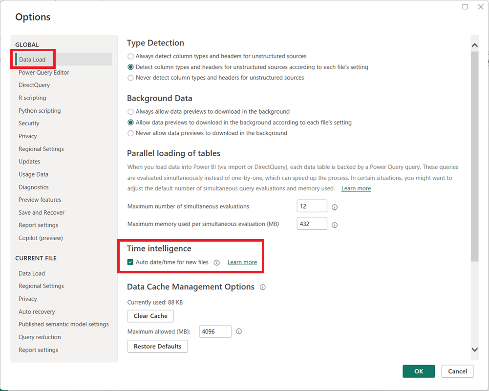
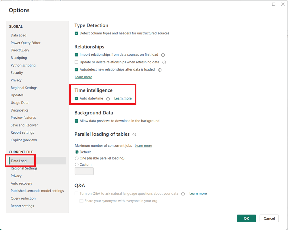
Power BI includes a feature called Auto date/time that automatically creates hidden date tables for date columns in your model. While this can be helpful for quick analyses, it can also introduce performance issues and modeling complexity in more advanced or production-grade reports.
What Is Auto Date/Time?
When Auto date/time is enabled, Power BI automatically generates a hidden date table for every column of type Date or Date/Time. These tables allow you to use built-in time intelligence features (like Year, Quarter, and Month) without explicitly creating a calendar table.
Why Turn Off Auto Date/Time?
Disabling Auto date/time is often considered a best practice for the following reasons:
Better Performance Each date column gets its own hidden date table, which increases model size and can slow down report performance.
Cleaner Data Models Hidden tables can clutter the model and make debugging DAX calculations more difficult.
Consistent Time Intelligence Using a single, well-designed Date (Calendar) table ensures consistent logic across all measures and visuals.
More Control Custom calendar tables allow you to define fiscal years, custom week logic, holidays, and other business-specific requirements.
How to Turn Off Auto Date/Time in Power BI
You can disable Auto date/time in both Power BI Desktop and at the report level:
In Power BI Desktop, go to File → Options and settings → Options.
Under Global, select Data Load.
Uncheck Auto date/time for new files.
(Optional but recommended) Under Current File, select Data Load and uncheck Auto date/time to disable it for the current report.
Click OK and refresh your model if necessary.
When Should You Leave It On?
Auto date/time can still be useful for:
Quick prototypes or ad-hoc analysis
Simple models with only one or two date fields
Users new to Power BI who are not yet working with custom DAX time intelligence
Final Thoughts
For enterprise, reusable, or performance-sensitive Power BI models, turning off Auto date/time and using a dedicated Date table is usually the better approach. It leads to cleaner models, more reliable calculations, and greater long-term flexibility as your reports grow in complexity.
This is your one-stop hub with information for preparing for the DP-600: Implementing Analytics Solutions Using Microsoft Fabric certification exam. Upon successful completion of the exam, you earn the Fabric Analytics Engineer Associate certification.
This hub provides information directly here, links to a number of external resources, tips for preparing for the exam, practice tests, and section questions to help you prepare. Bookmark this page and use it as a guide to ensure that you are fully covering all relevant topics for the exam and using as many of the resources available as possible. We hope you find it convenient and helpful.
Why do the DP-600: Implementing Analytics Solutions Using Microsoft Fabric exam to gain the Fabric Analytics Engineer Associate certification?
Most likely, you already know why you want to earn this certification, but in case you are seeking information on its benefits, here are a few: (1) there is a possibility for career advancement because Microsoft Fabric is a leading data platform used by companies of all sizes, all over the world, and is likely to become even more popular (2) greater job opportunities due to the edge provided by the certification (3) higher earnings potential, (4) you will expand your knowledge about the Fabric platform by going beyond what you would normally do on the job and (5) it will provide immediate credibility about your knowledge, and (6) it may, and it should, provide you with greater confidence about your knowledge and skills.
Important DP-600 resources:
In the section below this one, titled “DP-600: Skills measured as of October 31, 2025“, you will find the “skills measured” topics from the official study guide with links to exam preparation content for each topic. Bookmark this page and use that section as a structured topic-by-topic guide for your prep.
This page provides information for preparing for, practicing for, and registering for the exam. The skills measured content in the guide is also what is used to form the “Skills Measured as of …” outline below.
About the exam:
Cost: US $165
Number of questions: approximately 60
Time to do exam: 120 minutes (2 hours)
To Do’s:
Schedule time to learn, study, perform labs, and do practice exams and questions
Schedule the exam based on when you think you will be ready; scheduling the exam gives you a target and drives you to keep working on it
Use the various resources above and below to learn
Take the free Microsoft Learn practice test, any other available practice tests, and do the practice questions in each section and the two practice tests available in this hub.
Link to the free, comprehensive, self-paced course: Microsoft Learn course for a Microsoft Fabric Analytics Engineer. It contains 4 Learning Paths, each with multiple Modules, and each module has multiple Units. It will take some time to do it, but we recommend that you complete this entire course, including the exercises/labs. To help you work through your preparation in a structured manner, we will point you to the relevant sections in the training material corresponding to each of the sections in the skills measured section below.
Here you can learn in a structured manner by going through the topics of the exam one-by-one to ensure full coverage; click on each hyperlinked topic below to go to more information about it:
Good luck to you passing the DP-600: Implementing Analytics Solutions Using Microsoft Fabric certification exam and earning the Fabric Analytics Engineer Associate certification!
This post is a part of the DP-600: Implementing Analytics Solutions Using Microsoft Fabric Exam Prep Hub; and this topic falls under these sections:
Implement and manage semantic models (25-30%)
    --> Optimize enterprise-scale semantic models
        --> Implement performance improvements in queries and report visuals
Performance optimization is a critical skill for the Fabric Analytics Engineer. In enterprise-scale semantic models, poor query design, inefficient DAX, or overly complex visuals can significantly degrade report responsiveness and user experience. This exam section focuses on identifying performance bottlenecks and applying best practices to improve query execution, model efficiency, and report rendering.
1. Understand Where Performance Issues Occur
Performance problems typically fall into three layers:
a. Data & Storage Layer
Storage mode (Import, DirectQuery, Direct Lake, Composite)
Data source latency
Table size and cardinality
Partitioning and refresh strategies
b. Semantic Model & Query Layer
DAX calculation complexity
Relationships and filter propagation
Aggregation design
Use of calculation groups and measures
c. Report & Visual Layer
Number and type of visuals
Cross-filtering behavior
Visual-level queries
Use of slicers and filters
DP-600 questions often test your ability to identify the correct layer where optimization is needed.
2. Optimize Queries and Semantic Model Performance
a. Choose the Appropriate Storage Mode
Use Import for small-to-medium datasets requiring fast interactivity
Use Direct Lake for large OneLake Delta tables with high concurrency
Use Composite models to balance performance and real-time access
Avoid unnecessary DirectQuery when Import or Direct Lake is feasible
b. Reduce Data Volume
Remove unused columns and tables
Reduce column cardinality (e.g., avoid high-cardinality text columns)
Prefer surrogate keys over natural keys
Disable Auto Date/Time when not needed
c. Optimize Relationships
Use single-direction relationships by default
Avoid unnecessary bidirectional filters
Ensure relationships follow a star schema
Avoid many-to-many relationships unless required
d. Use Aggregations
Create aggregation tables to pre-summarize large fact tables
Enable query hits against aggregation tables before scanning detailed data
Especially valuable in composite models
3. Improve DAX Query Performance
a. Write Efficient DAX
Prefer measures over calculated columns
Use variables (VAR) to avoid repeated calculations
Minimize row context where possible
Avoid excessive iterators (SUMX, FILTER) over large tables
b. Use Filter Context Efficiently
Prefer CALCULATE with simple filters
Avoid complex nested FILTER expressions
Use KEEPFILTERS and REMOVEFILTERS intentionally
c. Avoid Expensive Patterns
Avoid EARLIER in favor of variables
Avoid dynamic table generation inside visuals
Minimize use of ALL when ALLSELECTED or scoped filters suffice
4. Optimize Report Visual Performance
a. Reduce Visual Complexity
Limit the number of visuals per page
Avoid visuals that generate multiple queries (e.g., complex custom visuals)
Use summary visuals instead of detailed tables where possible
b. Control Interactions
Disable unnecessary visual interactions
Avoid excessive cross-highlighting
Use report-level filters instead of visual-level filters when possible
c. Optimize Slicers
Avoid slicers on high-cardinality columns
Use dropdown slicers instead of list slicers
Limit the number of slicers on a page
d. Prefer Measures Over Visual Calculations
Avoid implicit measures created by dragging numeric columns
Define explicit measures in the semantic model
Reuse measures across visuals to improve cache efficiency
5. Use Performance Analysis Tools
a. Performance Analyzer
Identify slow visuals
Measure DAX query duration
Distinguish between query time and visual rendering time
b. Query Diagnostics (Power BI Desktop)
Analyze backend query behavior
Identify expensive DirectQuery or Direct Lake operations
c. DAX Studio (Advanced)
Analyze query plans
Measure storage engine vs formula engine time
Identify inefficient DAX patterns
(You won’t be tested on tool UI details, but knowing when and why to use them is exam-relevant.)
6. Common DP-600 Exam Scenarios
You may be asked to:
Identify why a report is slow and choose the best optimization
Identify the bottleneck layer (model, query, or visual)
Select the most appropriate storage mode for performance
Choose the least disruptive, most effective optimization
Improve a slow DAX measure
Reduce visual rendering time without changing the data source
Optimize performance for enterprise-scale models
Apply enterprise-scale best practices, not just quick fixes
Key Exam Takeaways
Always optimize the model first, visuals second
Star schema + clean relationships = better performance
Efficient DAX matters more than clever DAX
Fewer visuals and interactions = faster reports
Aggregations and Direct Lake are key enterprise-scale tools
This post is a part of the DP-600: Implementing Analytics Solutions Using Microsoft Fabric Exam Prep Hub; and this topic falls under these sections:
Implement and manage semantic models (25-30%)
    --> Design and build semantic models
        --> Identify use cases for and configure large semantic model storage format
Overview
As datasets grow in size and complexity, standard semantic model storage can become a limiting factor. Microsoft Fabric (via Power BI semantic models) provides a Large Semantic Model storage format designed to support very large datasets, higher cardinality columns, and more demanding analytical workloads.
For the DP-600 exam, you are expected to understand when to use large semantic models, what trade-offs they introduce, and how to configure them correctly.
What Is the Large Semantic Model Storage Format?
The Large semantic model option changes how data is stored and managed internally by the VertiPaq engine to support:
Larger data volumes (beyond typical in-memory limits)
Higher column cardinality
Improved scalability for enterprise workloads
This setting is especially relevant in Fabric Lakehouse and Warehouse-backed semantic models where data size can grow rapidly.
Key Characteristics
Designed for enterprise-scale models
Supports very large tables and partitions
Optimized for memory management, not raw speed
Works best with Import mode or Direct Lake
Requires Premium capacity or Fabric capacity
Common Use Cases
1. Very Large Fact Tables
Use large semantic models when:
Fact tables contain hundreds of millions or billions of rows
Historical data is retained for many years
Aggregations alone are not sufficient
2. High-Cardinality Columns
Ideal when models include:
Transaction IDs
GUIDs
Timestamps at high granularity
User or device identifiers
Standard storage can struggle with memory pressure in these scenarios.
3. Enterprise-Wide Shared Semantic Models
Useful for:
Centralized datasets reused across many reports
Models serving hundreds or thousands of users
Organization-wide KPIs and analytics
4. Complex Models with Many Tables
When your model includes:
Numerous dimension tables
Multiple fact tables
Complex relationships
Large storage format improves stability and scalability.
5. Direct Lake Models Over OneLake
In Microsoft Fabric:
Large semantic models pair well with Direct Lake
Enable querying massive Delta tables without full data import
Reduce duplication of data between OneLake and the model
When NOT to Use Large Semantic Models
Avoid using large semantic models when:
The dataset is small or moderate in size
Performance is more critical than scalability
The model is used by a limited number of users
You rely heavily on fast interactive slicing
For smaller models, standard storage often provides better query performance.
Performance Trade-Offs
Aspect
Standard Storage
Large Storage
Memory efficiency
Moderate
High
Query speed
Faster
Slightly slower
Max model size
Limited
Much larger
Cardinality tolerance
Lower
Higher
Enterprise scalability
Limited
High
Exam Tip: Large semantic models favor scalability over speed.
How to Configure Large Semantic Model Storage Format
Prerequisites
Fabric capacity or Power BI Premium
Import or Direct Lake storage mode
Dataset ownership permissions
Configuration Steps
Open Power BI Desktop
Go to Model view
Select the semantic model
In Model properties, locate Large dataset storage
Enable the option
Publish the model to Fabric or Power BI Service
Once enabled, the setting cannot be reverted back to standard storage.
Important Configuration Considerations
Enable before model grows significantly
Combine with:
Partitioning
Aggregation tables
Proper star schema design
Monitor memory usage in capacity metrics
Plan refresh strategies carefully
Relationship to DP-600 Exam Topics
This section connects directly with:
Storage mode selection
Semantic model scalability
Direct Lake and OneLake integration
Enterprise model design decisions
Expect scenario-based questions asking you to choose the appropriate storage format based on:
Data volume
Cardinality
Performance requirements
Capacity constraints
Key Takeaways for the Exam
Large semantic models support very large, complex datasets
Use large semantic models for scale, not speed
Best for enterprise-scale analytics
Ideal for high-cardinality, high-volume, enterprise models
Trade performance for scalability
Require Premium or Fabric capacity
One-way configuration—so, plan ahead
Often paired/combined with Direct Lake
Practice Questions:
Here are 10 questions to test and help solidify your learning and knowledge. As you review these and other questions in your preparation, make sure to …
Identifying and understand why an option is correct (or incorrect) — not just which one
Look for and understand the usage scenario of keywords in exam questions to guide you
Expect scenario-based questions rather than direct definitions
1. When should you enable the large semantic model storage format?
A. When the model is used by a small number of users B. When the dataset contains very large fact tables and high-cardinality columns C. When query performance must be maximized for small datasets D. When using Import mode with small dimension tables
Correct Answer: B
Explanation: Large semantic models are designed to handle very large datasets and high-cardinality columns. Small or simple models do not benefit and may experience reduced performance.
2. Which storage modes support large semantic model storage format?
A. DirectQuery only B. Import and Direct Lake C. Live connection only D. All Power BI storage modes
Correct Answer: B
Explanation: Large semantic model storage format is supported with Import and Direct Lake modes. It is not applicable to Live connections or DirectQuery-only scenarios.
3. What is a primary trade-off when using large semantic model storage format?
A. Increased query speed B. Reduced memory usage with no downsides C. Slightly slower query performance in exchange for scalability D. Loss of DAX functionality
Correct Answer: C
Explanation: Large semantic models favor scalability and memory efficiency over raw query speed, which can be slightly slower compared to standard storage.
4. Which scenario is the best candidate for a large semantic model?
A. A departmental sales report with 1 million rows B. A personal Power BI report with static data C. An enterprise model with billions of transaction records D. A DirectQuery model against a SQL database
Correct Answer: C
Explanation: Large semantic models are ideal for enterprise-scale datasets with very large row counts and complex analytics needs.
5. What happens after enabling large semantic model storage format?
A. It can be disabled at any time B. The model automatically switches to DirectQuery C. The setting cannot be reverted D. Aggregation tables are created automatically
Correct Answer: C
Explanation: Once enabled, large semantic model storage format cannot be turned off, making early planning important.
6. Which capacity requirement applies to large semantic models?
A. Power BI Free B. Power BI Pro C. Power BI Premium or Microsoft Fabric capacity D. Any capacity type
Correct Answer: C
Explanation: Large semantic models require Premium capacity or Fabric capacity due to their increased resource demands.
7. Why are high-cardinality columns a concern in standard semantic models?
A. They prevent relationships from being created B. They increase memory usage and reduce compression efficiency C. They disable aggregations D. They are unsupported in Power BI
Correct Answer: B
Explanation: High-cardinality columns reduce VertiPaq compression efficiency, increasing memory pressure—one reason to use large semantic model storage.
8. Which Fabric feature commonly pairs with large semantic models for massive datasets?
A. Power Query Dataflows B. DirectQuery C. Direct Lake over OneLake D. Live connection to Excel
Correct Answer: C
Explanation: Large semantic models pair well with Direct Lake, allowing efficient querying of large Delta tables stored in OneLake.
9. Which statement best describes large semantic model performance?
A. Always faster than standard storage B. Optimized for small, interactive datasets C. Optimized for scalability and memory efficiency D. Not compatible with DAX calculations
Correct Answer: C
Explanation: Large semantic models prioritize scalability and efficient memory management, not maximum query speed.
10. Which design practice should accompany large semantic models?
A. Flat denormalized tables only B. Star schema, aggregations, and partitioning C. Avoid relationships entirely D. Disable incremental refresh
Correct Answer: B
Explanation: Best practices such as star schema design, aggregation tables, and partitioning are critical for maintaining performance and manageability in large semantic models.
This post is a part of the DP-600: Implementing Analytics Solutions Using Microsoft Fabric Exam Prep Hub; and this topic falls under these sections:
Implement and manage semantic models (25-30%)
    --> Design and build semantic models
        --> Write calculations that use DAX variables and functions, such as
            iterators, table filtering, windowing, and information functions
Why This Topic Matters for DP-600
DAX (Data Analysis Expressions) is the core language used to define business logic in Power BI and Fabric semantic models. The DP-600 exam emphasizes not just basic aggregation, but the ability to:
Write readable, efficient, and maintainable measures
Control filter context and row context
Use advanced DAX patterns for real-world analytics
Understanding variables, iterators, table filtering, windowing, and information functions is essential for building performant and correct semantic models.
Using DAX Variables (VAR)
What Are DAX Variables?
DAX variables allow you to:
Store intermediate results
Avoid repeating calculations
Improve readability and performance
Syntax
VAR VariableName = Expression
RETURN FinalExpression
Example
Total Sales (High Value) =
VAR Threshold = 100000
VAR TotalSales = SUM(FactSales[SalesAmount])
RETURN
IF(TotalSales > Threshold, TotalSales, BLANK())
Benefits of Variables
Evaluated once per filter context
Improve performance
Make complex logic easier to debug
Exam Tip: Expect questions asking why variables are preferred over repeated expressions.
Iterator Functions
What Are Iterators?
Iterators evaluate an expression row by row over a table, then aggregate the results.
Common Iterators
Function
Purpose
SUMX
Row-by-row sum
AVERAGEX
Row-by-row average
COUNTX
Row-by-row count
MINX / MAXX
Row-by-row min/max
Example
Total Line Sales =
SUMX(
    FactSales,
    FactSales[Quantity] * FactSales[UnitPrice]
)
Key Concept
Iterators create row context
Often combined with CALCULATE and FILTER
Table Filtering Functions
FILTER
Returns a table filtered by a condition.
High Value Sales =
CALCULATE(
    SUM(FactSales[SalesAmount]),
    FILTER(
        FactSales,
        FactSales[SalesAmount] > 1000
    )
)
Related Functions
Function
Purpose
FILTER
Row-level filtering
ALL
Remove filters
ALLEXCEPT
Remove filters except specified columns
VALUES
Distinct values in current context
Exam Tip: Understand how FILTER interacts with CALCULATE and filter context.
Windowing Functions
Windowing functions enable calculations over ordered sets of rows, often used for time intelligence and ranking.
Exam Note: Windowing functions are increasingly emphasized in modern DAX patterns.
Information Functions
Information functions return metadata or context information rather than numeric aggregations.
Common Information Functions
Function
Purpose
ISFILTERED
Detects column filtering
HASONEVALUE
Checks if a single value exists
SELECTEDVALUE
Returns value if single selection
ISBLANK
Checks for blank results
Example
Selected Year =
IF(
    HASONEVALUE(DimDate[Year]),
    SELECTEDVALUE(DimDate[Year]),
    "Multiple Years"
)
Use Cases
Dynamic titles
Conditional logic in measures
Debugging filter context
Combining These Concepts
Real-world DAX often combines multiple techniques:
Average Monthly Sales =
VAR MonthlySales =
    SUMX(
        VALUES(DimDate[Month]),
        [Total Sales]
    )
RETURN
AVERAGEX(
    VALUES(DimDate[Month]),
    MonthlySales
)
This example uses:
Variables
Iterators
Table functions
Filter context awareness
Performance Considerations
Prefer variables over repeated expressions
Minimize complex iterators over large fact tables
Use star schemas to simplify DAX
Avoid unnecessary row context when simple aggregation works
Common Exam Scenarios
You may be asked to:
Identify the correct use of SUM vs SUMX
Choose when to use FILTER vs CALCULATE
Interpret the effect of variables on evaluation
Diagnose incorrect ranking or aggregation results
Correct answers typically emphasize:
Clear filter context
Efficient evaluation
Readable and maintainable DAX
Best Practices Summary
Use VAR / RETURN for complex logic
Use iterators only when needed
Control filter context explicitly
Leverage information functions for conditional logic
Test measures under multiple filter scenarios
Quick Exam Tips
VAR / RETURN = clarity + performance
SUMX ≠ SUM (row-by-row vs column aggregation)
CALCULATE = filter context control
RANKX / WINDOW = ordered analytics
SELECTEDVALUE = safe single-selection logic
Summary
Advanced DAX calculations are foundational to effective semantic models in Microsoft Fabric:
Variables improve clarity and performance
Iterators enable row-level logic
Table filtering controls context precisely
Windowing functions support advanced analytics
Information functions make models dynamic and robust
Mastering these patterns is essential for both real-world analytics and DP-600 exam success.
Practice Questions:
Here are 10 questions to test and help solidify your learning and knowledge. As you review these and other questions in your preparation, make sure to …
Identifying and understand why an option is correct (or incorrect) — not just which one
Look for and understand the usage scenario of keywords in exam questions to guide you
Expect scenario-based questions rather than direct definitions
1. What is the primary benefit of using DAX variables (VAR)?
A. They change row context to filter context B. They improve readability and reduce repeated calculations C. They enable bidirectional filtering D. They create calculated columns dynamically
Correct Answer: B
Explanation: Variables store intermediate results that are evaluated once per filter context, improving performance and readability.
2. Which function should you use to perform row-by-row calculations before aggregation?
A. SUM B. CALCULATE C. SUMX D. VALUES
Correct Answer: C
Explanation: SUMX is an iterator that evaluates an expression row by row before summing the results.
3. Which statement best describes the FILTER function?
A. It modifies filter context without returning a table B. It returns a table filtered by a logical expression C. It aggregates values across rows D. It converts row context into filter context
Correct Answer: B
Explanation: FILTER returns a table and is commonly used inside CALCULATE to apply row-level conditions.
4. What happens when CALCULATE is used in a measure?
A. It creates a new row context B. It permanently changes relationships C. It modifies the filter context D. It evaluates expressions only once
Correct Answer: C
Explanation: CALCULATE evaluates an expression under a modified filter context and is central to most advanced DAX logic.
5. Which function is most appropriate for ranking values in a table?
A. COUNTX B. WINDOW C. RANKX D. OFFSET
Correct Answer: C
Explanation: RANKX assigns a ranking to each row based on an expression evaluated over a table.
6. What is a common use case for windowing functions such as OFFSET or WINDOW?
A. Creating relationships B. Detecting blank values C. Calculating running totals or moving averages D. Removing duplicate rows
Correct Answer: C
Explanation: Windowing functions operate over ordered sets of rows, making them ideal for time-based analytics.
7. Which information function returns a value only when exactly one value is selected?
A. HASONEVALUE B. ISFILTERED C. SELECTEDVALUE D. VALUES
Correct Answer: C
Explanation: SELECTEDVALUE returns the value when a single value exists in context; otherwise, it returns blank or a default.
8. When should you prefer SUM over SUMX?
A. When calculating expressions row by row B. When multiplying columns C. When aggregating a single numeric column D. When filter context must be modified
Correct Answer: C
Explanation: SUM is more efficient when simply adding values from one column without row-level logic.
9. Why can excessive use of iterators negatively impact performance?
A. They ignore filter context B. They force bidirectional filtering C. They evaluate expressions row by row D. They prevent column compression
Correct Answer: C
Explanation: Iterators process each row individually, which can be expensive on large fact tables.
10. Which combination of DAX concepts is commonly used to build advanced, maintainable measures?
A. Variables and relationships B. Iterators and calculated columns C. Variables, CALCULATE, and table functions D. Information functions and bidirectional filters
Correct Answer: C
Explanation: Advanced DAX patterns typically combine variables, CALCULATE, and table functions for clarity and performance.
This post is a part of the DP-600: Implementing Analytics Solutions Using Microsoft Fabric Exam Prep Hub; and this topic falls under these sections:
Implement and manage semantic models (25-30%)
    --> Design and build semantic models
        --> Implement Relationships, Such as Bridge Tables
            and Many-to-Many Relationships
Why Relationships Matter in Semantic Models
In Microsoft Fabric and Power BI semantic models, relationships define how tables interact and how filters propagate across data. Well-designed relationships are critical for:
Accurate aggregations
Predictable filtering behavior
Correct DAX calculations
Optimal query performance
While one-to-many relationships are preferred, real-world data often requires handling many-to-many relationships using techniques such as bridge tables.
Common Relationship Types in Semantic Models
1. One-to-Many (Preferred)
One dimension row relates to many fact rows
Most common and performant relationship
Typical in star schemas
Example:
DimCustomer → FactSales
2. Many-to-Many
Multiple rows in one table relate to multiple rows in another
More complex filtering behavior
Can negatively impact performance if not modeled correctly
Example:
Customers associated with multiple regions
Products assigned to multiple categories
Understanding Many-to-Many Relationships
Native Many-to-Many Relationships
Power BI supports direct many-to-many relationships, but these should be used carefully.
Characteristics:
Cardinality: Many-to-many
Filters propagate ambiguously
DAX becomes harder to reason about
Exam Tip: Direct many-to-many relationships are supported but not always recommended for complex models.
Bridge Tables (Best Practice)
A bridge table (also called a factless fact table) resolves many-to-many relationships by introducing an intermediate table.
What Is a Bridge Table?
A table that:
Contains keys from two related entities
Has no numeric measures
Enables controlled filtering paths
Example Scenario
Business case: Products can belong to multiple categories.
Tables:
DimProduct (ProductID, Name)
DimCategory (CategoryID, CategoryName)
BridgeProductCategory (ProductID, CategoryID)
Relationships:
DimProduct → BridgeProductCategory (one-to-many)
DimCategory → BridgeProductCategory (one-to-many)
This converts a many-to-many relationship into two one-to-many relationships.
Benefits of Using Bridge Tables
Benefit
Description
Predictable filtering
Clear filter paths
Better DAX control
Easier to write and debug measures
Improved performance
Avoids ambiguous joins
Scalability
Handles complex relationships cleanly
Filter Direction Considerations
Single vs Bidirectional Filters
Single direction (recommended): Filters flow from dimension → bridge → fact
Bidirectional: Can simplify some scenarios but increases ambiguity
Exam Guidance:
Use single-direction filters by default
Enable bidirectional filtering only when required and understood
Many-to-Many and DAX Implications
When working with many-to-many relationships:
Measures may return unexpected results
DISTINCTCOUNT is commonly required
Explicit filtering using DAX functions may be necessary
Common DAX patterns:
CALCULATE
TREATAS
CROSSFILTER (advanced)
Relationship Best Practices for DP-600
Favor star schemas with one-to-many relationships
Use bridge tables instead of direct many-to-many when possible
Avoid unnecessary bidirectional filters
Validate relationship cardinality and direction
Test measures under different filtering scenarios
Common Exam Scenarios
You may see questions like:
“How do you model a relationship where products belong to multiple categories?”
“What is the purpose of a bridge table?”
“What are the risks of many-to-many relationships?”
Correct answers typically emphasize:
Bridge tables
Controlled filter propagation
Avoiding ambiguous relationships
Star Schema vs Many-to-Many Models
Feature
Star Schema
Many-to-Many
Complexity
Low
Higher
Performance
Better
Lower
DAX simplicity
High
Lower
Use cases
Most analytics
Specialized scenarios
Summary
Implementing relationships correctly is foundational to building reliable semantic models in Microsoft Fabric:
One-to-many relationships are preferred
Many-to-many relationships should be handled carefully
Bridge tables provide a scalable, exam-recommended solution
Clear relationships lead to accurate analytics and simpler DAX
Exam Tip
If a question involves multiple entities relating to each other, or many-to-many relationships, the most likely answer usually includes using a “bridge table”.
Practice Questions:
Here are 10 questions to test and help solidify your learning and knowledge. As you review these and other questions in your preparation, make sure to …
Identifying and understand why an option is correct (or incorrect) — not just which one
Look for and understand the usage scenario of keywords in exam questions to guide you
Expect scenario-based questions rather than direct definitions
1. Which relationship type is generally preferred in Power BI semantic models?
A. Many-to-many B. One-to-one C. One-to-many D. Bidirectional many-to-many
Correct Answer: C
Explanation: One-to-many relationships provide predictable filter propagation, better performance, and simpler DAX calculations.
2. What is the primary purpose of a bridge table?
A. Store aggregated metrics B. Normalize dimension attributes C. Resolve many-to-many relationships D. Improve data refresh performance
Correct Answer: C
Explanation: Bridge tables convert many-to-many relationships into two one-to-many relationships, improving model clarity and control.
3. Which characteristic best describes a bridge table?
A. Contains numeric measures B. Stores transactional data C. Contains keys from related tables only D. Is always filtered bidirectionally
Correct Answer: C
Explanation: Bridge tables typically contain only keys (foreign keys) and no measures, enabling relationship resolution.
4. What is a common risk of using native many-to-many relationships directly?
A. They cannot be refreshed B. They cause data duplication C. They create ambiguous filter propagation D. They are unsupported in Fabric
Correct Answer: C
Explanation: Native many-to-many relationships can result in ambiguous filtering and unpredictable aggregation results.
5. In a bridge table scenario, how are relationships typically defined?
A. Many-to-many on both sides B. One-to-one from both dimensions C. One-to-many from each dimension to the bridge D. Bidirectional many-to-one
Correct Answer: C
Explanation: Each dimension connects to the bridge table using a one-to-many relationship.
6. When should bidirectional filtering be enabled?
A. Always, for simplicity B. Only when necessary and well-understood C. Only on fact tables D. Never in semantic models
Correct Answer: B
Explanation: Bidirectional filters can be useful but introduce complexity and ambiguity if misused.
7. Which scenario is best handled using a bridge table?
A. A customer has one address B. A sale belongs to one product C. A product belongs to multiple categories D. A date table relates to a fact table
Correct Answer: C
Explanation: Products belonging to multiple categories is a classic many-to-many scenario requiring a bridge table.
8. How does a properly designed bridge table affect DAX measures?
A. Makes measures harder to write B. Requires custom SQL logic C. Enables predictable filter behavior D. Eliminates the need for CALCULATE
Correct Answer: C
Explanation: Bridge tables create clear filter paths, making DAX behavior more predictable and reliable.
9. Which DAX function is commonly used to handle complex many-to-many filtering scenarios?
A. SUMX B. RELATED C. TREATAS D. LOOKUPVALUE
Correct Answer: C
Explanation: TREATAS is often used to apply filters across tables that are not directly related.
10. For DP-600 exam questions involving many-to-many relationships, which solution is typically preferred?
A. Direct many-to-many relationships B. Denormalized fact tables C. Bridge tables with one-to-many relationships D. Duplicate dimension tables
Correct Answer: C
Explanation: The exam emphasizes scalable, maintainable modeling practices — bridge tables are the recommended solution.
Dimension tables store contextual attributes that describe facts.
Examples:
Customer (name, segment, region)
Product (category, brand)
Date (calendar attributes)
Store or location
Characteristics:
Typically smaller than fact tables
Used to filter and group measures
Building a Star Schema for a Semantic Model
1. Identify the Grain of the Fact Table
The grain defines the level of detail in the fact table — for example:
One row per sales transaction per customer per day
Understand the grain before building dimensions.
2. Design Dimension Tables
Dimensions should be:
Descriptive
De-duplicated
Hierarchical where relevant (e.g., Country > State > City)
Example:
DimProduct
DimCustomer
DimDate
ProductID
CustomerID
DateKey
Name
Name
Year
Category
Segment
Quarter
Brand
Region
Month
3. Define Relationships
Semantic models should have clear relationships:
Fact → Dimension: one-to-many
No ambiguous cycles
Avoid overly complex circular relationships
In a star schema:
Fact table joins to each dimension
Dimensions do not join to each other directly
4. Import into Semantic Model
In Power BI Desktop or Fabric:
Load fact and dimension tables
Validate relationships
Ensure correct cardinality
Mark the Date dimension as a Date table if appropriate
Benefits in Semantic Modeling
Benefit
Description
Performance
Simplified relationships yield faster queries
Usability
Model is intuitive for report authors
Maintenance
Easier to document and manage
DAX Simplicity
Measures use clear filter paths
DAX and Star Schema
Star schemas make DAX measures more predictable:
Example measure:
Total Sales = SUM(FactSales[SalesAmount])
With a proper star schema:
Filtering by dimension (e.g., DimCustomer[Region] = “West”) automatically propagates to the fact table
DAX measure logic is clean and consistent
Star Schema vs Snowflake Schema
Feature
Star Schema
Snowflake Schema
Complexity
Simple
More complex
Query performance
Typically better
Slightly slower
Modeling effort
Lower
Higher
Normalization
Low
High
For analytical workloads (like in Fabric and Power BI), star schemas are generally preferred.
When to Apply a Star Schema
Use star schema design when:
You are building semantic models for BI/reporting
Data is sourced from multiple systems
You need to support slicing and dicing by multiple dimensions
Performance and maintainability are priorities
Semantic models built on star schemas work well with:
Import mode
Direct Lake with dimensional context
Composite models
Common Exam Scenarios
You might encounter questions like:
“Which table should be the fact in this model?”
“Why should dimensions be separated from fact tables?”
“How does a star schema improve performance in a semantic model?”
Key answers will focus on:
Simplified relationships
Better DAX performance
Intuitive filtering and slicing
Best Practices for Semantic Star Schemas
Explicitly define date tables and mark them as such
Avoid many-to-many relationships where possible
Keep dimensions denormalized (flattened)
Ensure fact tables have surrogate keys linking to dimensions
Validate cardinality and relationship directions
Exam Tip
If a question emphasizes performance, simplicity, clear filtering behavior, and ease of reporting, a star schema is likely the correct design choice / optimal answer.
Summary
Implementing a star schema for a semantic model is a proven best practice in analytics:
Central fact table
Descriptive dimensions
One-to-many relationships
Optimized for DAX and interactive reporting
This approach supports Fabric’s goal of providing fast, flexible, and scalable analytics.
Practice Questions:
Here are 10 questions to test and help solidify your learning and knowledge. As you review these and other questions in your preparation, make sure to …
Identifying and understand why an option is correct (or incorrect) — not just which one
Look for and understand the usage scenario of keywords in exam questions to guide you
Expect scenario-based questions rather than direct definitions
1. What is the primary purpose of a star schema in a semantic model?
A. To normalize data to reduce storage B. To optimize transactional workloads C. To simplify analytics and improve query performance D. To enforce row-level security
Correct Answer: C
Explanation: Star schemas are designed specifically for analytics. They simplify relationships and improve query performance by organizing data into fact and dimension tables.
2. In a star schema, what type of data is typically stored in a fact table?
A. Descriptive attributes such as names and categories B. Hierarchical lookup values C. Numeric measures related to business processes D. User-defined calculated columns
Correct Answer: C
Explanation: Fact tables store measurable, numeric values such as revenue, quantity, or counts, which are analyzed across dimensions.
3. Which relationship type is most common between fact and dimension tables in a star schema?
A. One-to-one B. One-to-many C. Many-to-many D. Bidirectional many-to-many
Correct Answer: B
Explanation: Each dimension record (e.g., a customer) can relate to many fact records (e.g., multiple sales), making one-to-many relationships standard.
4. Why are star schemas preferred over snowflake schemas in Power BI semantic models?
A. Snowflake schemas require more storage B. Star schemas improve DAX performance and model usability C. Snowflake schemas are not supported in Fabric D. Star schemas eliminate the need for relationships
Correct Answer: B
Explanation: Star schemas reduce relationship complexity, making DAX calculations simpler and improving query performance.
5. Which table should typically contain a DateKey column in a star schema?
A. Dimension tables only B. Fact tables only C. Both fact and dimension tables D. Neither table type
Correct Answer: C
Explanation: The fact table uses DateKey as a foreign key, while the Date dimension uses it as a primary key.
6. What is the “grain” of a fact table?
A. The number of rows in the table B. The level of detail represented by each row C. The number of dimensions connected D. The data type of numeric columns
Correct Answer: B
Explanation: Grain defines what a single row represents (e.g., one sale per customer per day).
7. Which modeling practice helps ensure optimal performance in a semantic model?
A. Creating relationships between dimension tables B. Using many-to-many relationships by default C. Keeping dimensions denormalized D. Storing text attributes in the fact table
Correct Answer: C
Explanation: Denormalized (flattened) dimension tables reduce joins and improve query performance in analytic models.
8. What happens when a dimension is used to filter a report in a properly designed star schema?
A. The filter applies only to the dimension table B. The filter automatically propagates to the fact table C. The filter is ignored by measures D. The filter causes a many-to-many relationship
Correct Answer: B
Explanation: Filters flow from dimension tables to the fact table through one-to-many relationships.
9. Which scenario is best suited for a star schema in a semantic model?
A. Real-time transactional processing B. Log ingestion with high write frequency C. Interactive reporting with slicing and aggregation D. Application-level CRUD operations
Correct Answer: C
Explanation: Star schemas are optimized for analytical queries involving aggregation, filtering, and slicing.
10. What is a common modeling mistake when implementing a star schema?
A. Using surrogate keys B. Creating direct relationships between dimension tables C. Marking a date table as a date table D. Defining one-to-many relationships
Correct Answer: B
Explanation: Dimensions should not typically relate to each other directly in a star schema, as this introduces unnecessary complexity.